
Orientation of the fiber suspending in the flow through a tube containing a sphere*
2013-06-01 12:29LIANGXiaoyu梁晓瑜
水动力学研究与进展 B辑 2013年2期
LIANG Xiao-yu (梁晓瑜)
Institute of Fluid Engineering, School of Aeronautics and Astronautics, Zhejiang University, Hangzhou 310027, China
College of Metrology and Measurement Engineering, China Jiliang University, Hangzhou 310018, China,
E-mail: liangxiaoyu002@sina.cn
KU Xiao-ke
Department of Energy and Process Engineering, Norwegian University of Science and Technology, Norwegian, Norway
WANG Ye-long (王叶龙)
Institute of Fluid Engineering, School of Aeronautics and Astronautics, Zhejiang University, Hangzhou 310027, China
Orientation of the fiber suspending in the flow through a tube containing a sphere*
LIANG Xiao-yu (梁晓瑜)
Institute of Fluid Engineering, School of Aeronautics and Astronautics, Zhejiang University, Hangzhou 310027, China
College of Metrology and Measurement Engineering, China Jiliang University, Hangzhou 310018, China,
E-mail: liangxiaoyu002@sina.cn
KU Xiao-ke
Department of Energy and Process Engineering, Norwegian University of Science and Technology, Norwegian, Norway
WANG Ye-long (王叶龙)
Institute of Fluid Engineering, School of Aeronautics and Astronautics, Zhejiang University, Hangzhou 310027, China
(Received June 27, 2012, Revised September 9, 2012)
Fiber suspensions flow through a tube containing a sphere in the dilute and concentrated regimes is simulated numerically with the Lattice Boltzmann Method (LBM). The numerical results of fiber orientation distribution based on a statistical scheme are obtained and agree qualitatively with the experimental ones for the flow through a parallel plate channel containing a cylinder. The results show that the sphere in the tube results in a change in the fiber orientation distribution downstream of the sphere along the flow and transverse directions. The influences of the sphere on the fiber orientation distribution are more significant for the concentrated suspensions than for the dilute one. The effect of the initial fiber orientations on the fiber orientation distribution is significant upstream of the sphere but small downstream of the sphere.
fiber suspension, laminar flow, tube containing a sphere, orientation distribution, Lattice Boltzmann Method (LBM)
Introduction
Fiber suspension occurs in a wide variety of natural and man-made materials. The orientation behavior of fibers is a major concern in many industrial processes, such as extrusion, injection, and compression molding. The fiber orientation distribution determines the mechanical, thermal and electrical properties of the fiber suspensions. In order to design and control manufacturing processes that generate favorable fiber orientation states, the description of the orientation pattern and the ways to control it must be well understood.
Over the past twenty years the fiber orientation distribution in the flow has been studied[1-4]. The main numerical methods for simulating the fiber orientation distribution include the Lttice Boltzmann Method (LBM)[5], the method of combining the slender body theory and the spectral method[6], and the Lagrangian method[7]. The LBM used in this study is a particletracing scheme. Application of the discrete Boltzmann method to analyze particles suspended in fluid was first proposed by Ladd et al.[8]. Ladd’s model requires fluid to cross the boundary of the suspended solid particle and occupy the entire domain. Aidun et al.[9]developed a method which does not require transfer of fluid into the solid particle and, therefore, applied to real suspension. Ding and Aidun[10]added“virtual nodes” to the solid boundaries and extended the LBM for direct simulation of suspended particles near con- tact. They also proposed a local link-by-link impleme- ntation of the lubrication force when the gapbetween spherical particles becomes very small. In the present study, the equations for fiber suspension in a Newtonian solvent are solved numerically by coupling flow field with fiber orientation. In the computation, the interactions between fibers, between fiber and cylinder in the channel, and between fiber and channel wall are taken into account.
Fiber orientation in a suspension flow through a tube is of scientific interest and is of importance in the actual application[11,12]. However, there are few studies[13,14]on the fiber orientation in flows through complex geometries. In the present study, we present a more complete model for the simulation of fiber orientation, and apply it to the computation of fiber orientation distributions in a flow through a tube containing a sphere. Such flow offers the possibilities of studying the behavior of the fibers in a variety of flows varying from simple shear or pure elongational flows, to more complex flows especially around the obstacle. Analyzing the flow in such geometry will beneficially contribute to reach a better understanding of flow properties in many important manufacturing processes of producing composites.
1. Numerical methods
1.1 Lattice Boltzmann Method
The original lattice Boltzmann equation in the discrete microscopic velocity space is given as
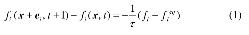
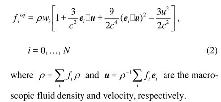
in which fiis the density distribution function,eiis the streaming velocity in the ithdirection in the phase space,i =0,1,… ,N,τis the single relaxation time, and fieqis the local equilibrium distribution and, for the square or cubic lattice, is taken as[15]
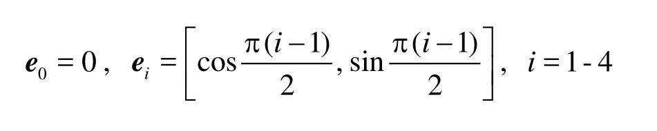
In the 9-bit LBGK model, two-dimensional velocity in the phase space is discretized in the following nine directions:
The kinematic viscosity for the nine-speed model is ν = c2Δt(τ -0.5)/3, and c =Δx /Δtis the lattice speed. In Eq.(2),wiis equal to 4/9 for i =0, 1/9 for i =1-4, and 1/36 for i=5-8.
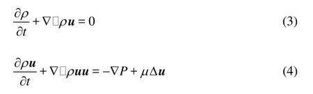
In the limit of long wavelengths, the LBE recovers the following quasi-incompressible N-S equations by the Chapman-Enskog multi-scaling expa-nsion[15]:
1.2 Force and torque exerted on fiber
The LBM has been a promising numerical tool to effectively model complex physics in computational fluid dynamics. Ladd et al.[8]and Aidun et al.[9]used the momentum exchange method to propose a modified bounce-back rule which is for a moving wall. We place the boundary nodes on the links connecting the interior and exterior nodes, then
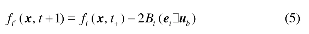
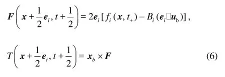
where “t+” denotes the post-collision time,iis the incident direction,i′is the reflected direction,Bi= 3ρwi/ c2,ubis the velocity on the particle surface,ub=u0+Ω×xb, where u0is the translational velocity of the mass center of the particle,Ωis the angular velocity of the particle, and xb= x+ei/2-x0with x0being the position of the mass center. The force and torque exerted by the fluid at xbare
1.3 Virtual fluid nodes
When simulating the discrete fibers, the LBM isusually limited to the case where the gap between fibers is much larger than the size of lattice unit. As the fibers get close to each other and the gap between them becomes smaller than a unit lattice dimension as shown in Fig.1, there is no fluid node within the gap. Thus two nodes on the gap link are covered by fibers and the LBM can not accurately calculate the hydrodynamic interaction between the fibers. In order to overcome this difficulty, Ding et al.[10]added “virtual nodes” to the boundaries and extended the LBM to the direct simulation of suspended fibers near contact. There are two fibers,IandJ , as shown in Fig.2. The initial point of link eiis nodex , just inside the boundary of fiber I , while the final point of link eiis nodey , just inside the boundary of fiberJ . Both nodes x and y are considered to be virtual fluid nodes. They serve as the real fluid nodes when the interaction between fiber I( J )and fluid in the gap area is being considered. Taking fiberI for example, the distribution function at nodex at time t +1on link eiis given by
wherei′always means the link with the direction opposite to that of linki,ubis the velocity of fiber I at x+ei/2, and Bi′=3ρwi′/c2. Consequently,the force and torque exerted on the fiberI by the node x are
where xb=x+ei/2-x0with x0being the position of centroid of fiberI.
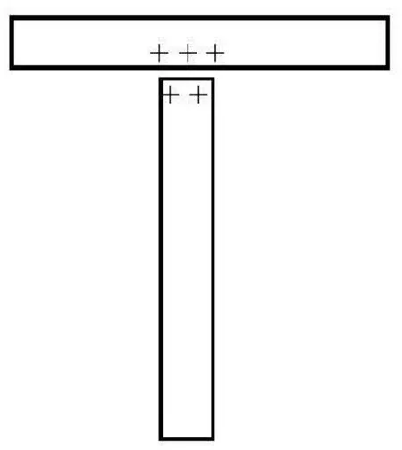
Fig.1 Two fibers with very small distance
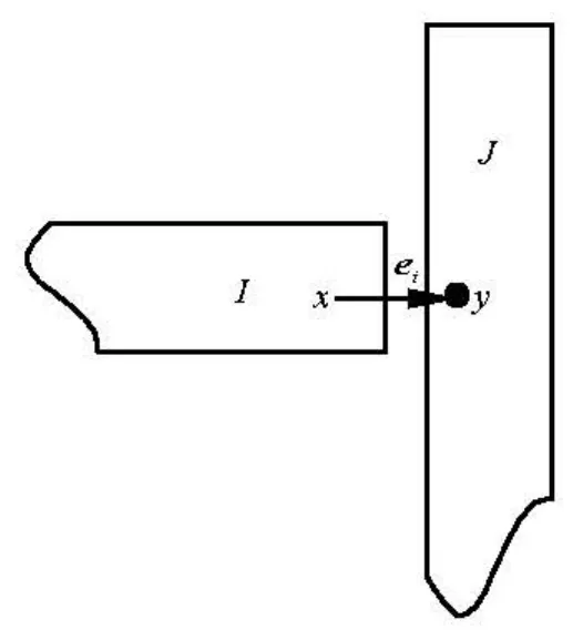
Fig.2 Interaction between two fibers near contact
The same rule is used to calculate the interaction between node y and fiberJ . When a fiber is very close to a wall, the interaction between the wall and the fiber is treated in a similar manner. Combining Eqs.(6) and (8), we have the total force and torque on the fiber during [t, t+1], excluding the lubrication force
1.4 Lubrication forces
To further represent the forces separating two fibers about to collide, the lubrication forces are included using links connecting two virtual boundary nodes from two surfaces near contact, defined as“bridge” links. The basic idea is to determine an element of force for each bridge link which accurately accounts for the lubrication force. The direction of the element of force is along the bridge link and given as d f =3ν ρU /2λ δ2, whereδis the surface separa
rtion,νis the kinematic viscosity,U is the relative velocity of the linked surface elements, and λrdepends on the surface curvature and is given by λr=(1/ R1+1/R2)/2for two spheres, where R1and R2are the radii of curvature of the linked two surface elements. It can be seen thatdf has a significant contribution to the lubrication force only when δis very small.df can be neglected ifδis larger than the length of the link. For two-dimensional case,df is given by
The force and the torque exerted on the particle along this link are given by
where xb= x+ ei/2-x0(x0is the position of the centroid of particle). So the total lubrication force and its torque exerted on a particle is then given by
If the fiber concentration is not too high, the end-toend or side-to-side proximity of two fibers rarely occurs. In most cases, the end of one fiber is close to the side of another one. Thus the lubrication approximation given above cannot be used if the fiber has a sharp edge. Therefore, we assume that the fibers have circular caps of diameterD (Dis the diameter of fiber) at their ends, and use the above lubrication approximation. When a fiber is very close to a wall, the fiber is treated in a similar manner.
From above equations, the net force and torque exerted on a fiber fromtto t +1are given by
The fiber velocity and angular velocity are updated based on Newton’s laws.
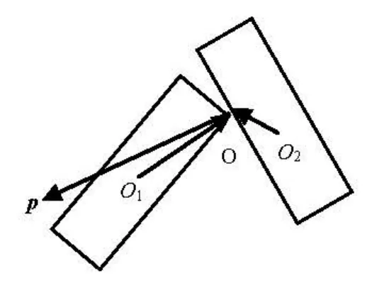
Fig.3 Collision model
2. Collision model
2.1 Collision between fibers
The collision of two fibers is assumed to be instantaneous and elastic. The contact point and its normal direction are determined by the relative positions of two fibers as shown in Fig.3. After collision, each fiber attains an impulse Ialong the normal direction. The translational and angular velocities of two fibers after collision depend on the impulse and are given as
where m and vare the mass and velocity of fiber, respectively,pis unit vector along the normal direction, the Subscripts 1 and 2 are used to distinguish two fibers, and the superscript ‘ ' ’means “after collision”. Based on the law of elastic collision, we have
where k is the elastic coefficient,v1Oand v2Oare the velocity components of two fibers along the normal direction at contact point before collision. The torques exerted on the two fibers arel1×Ipand -l2× Ip , respectively, where l1,l2are the vectors from mass centreO1and O2of two fibers to the contact pointO . Then the rotational equations of fibers are
where ωis the angular velocity of the fiber, and J1and J2are the rotation inertia of the fiber. Then the impulseI can be written as
2.2 Collision with wall or sphere
When fibers collide with wall or sphere, the model of collision between fibers is also used as long as taking m2as infinite and v2Oas 0. Then the transient impulse formula is obtained by reducing Eq.(17) to
3. Simulation details
3.1 Computational parameters

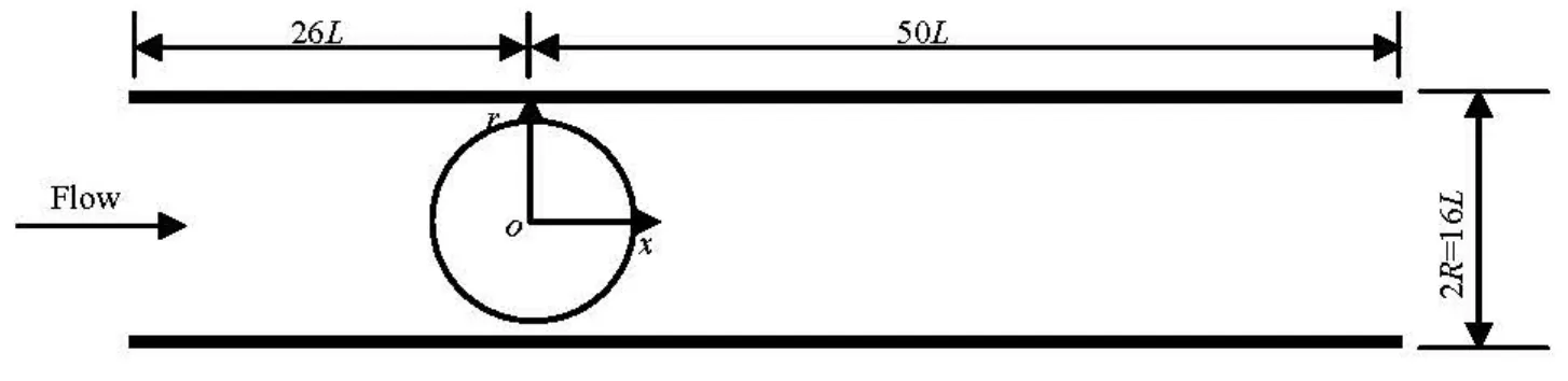
Fig.4 Schematic illustration of tube containing a sphere
3.2 Evolution of the orientation ellipses
In order to analyze the fiber orientation quantitatively, the flow region is divided into many small statistical cells (2L×1L). Then the second-order orientation tensorais calculated in each statistical cell from the orientation anglesθof fibers.θis defined as the angle between fiber axis and x-axis. The components of the tensora are given by
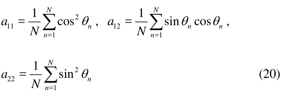
whereN and θnare the total number of fibers in each statistical cell and the orientation angle of each fiber, respectively. Whena12is equal to zero, the fiber axis coincides with the coordinate axis, and if furthermore,a11(or a22) is zero, the fibers are perfectly aligned with ther(orx) axis.
The preferred angleαof the fibers for each statistical cell is given by
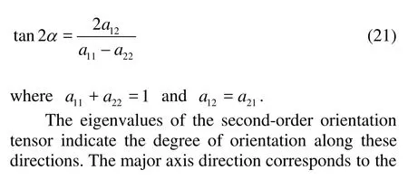
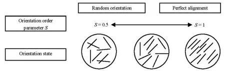
Fig.5 Illustration of the relation between the orientation state and the orientation parameters
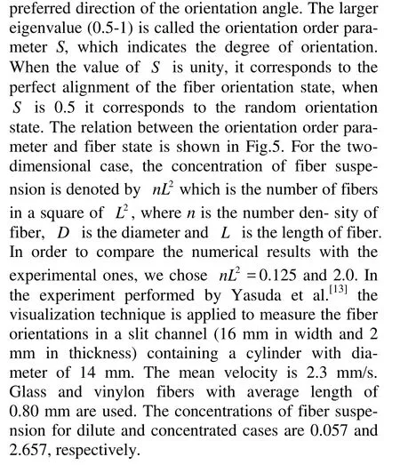
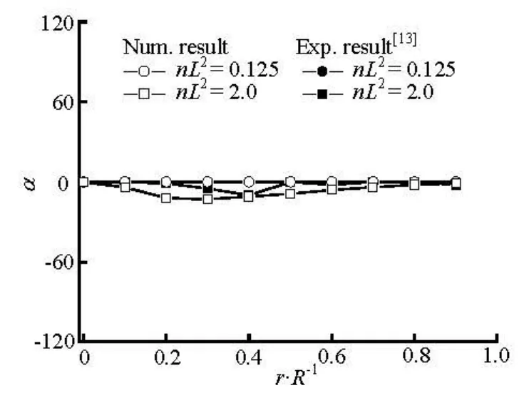
Fig.6 Distributions of preferred angle at x/ R =–2
4. Results and discussions
4.1 Orientation distributions of fibers along the radial direction
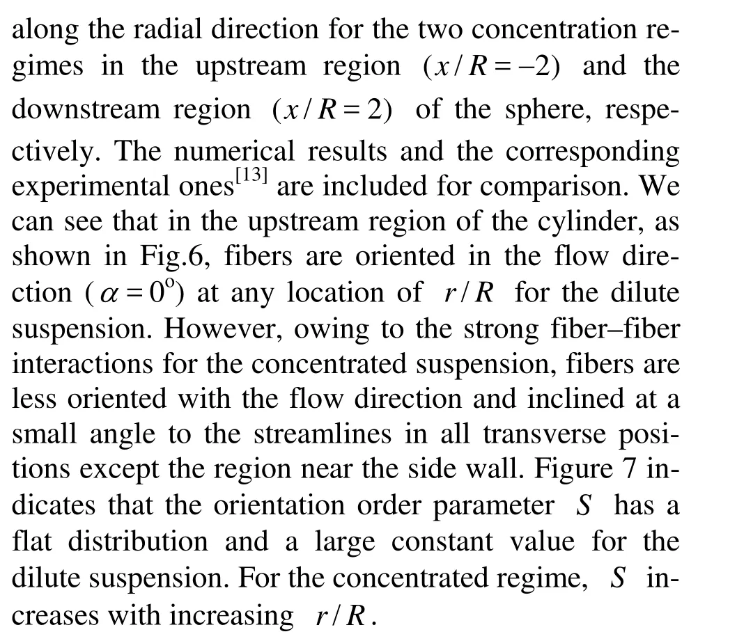
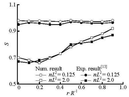
Fig.7 Distributions of orientation order parameter at x/ R=–2
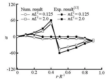
Fig.8 Distributions of preferred angle at x/ R =–2
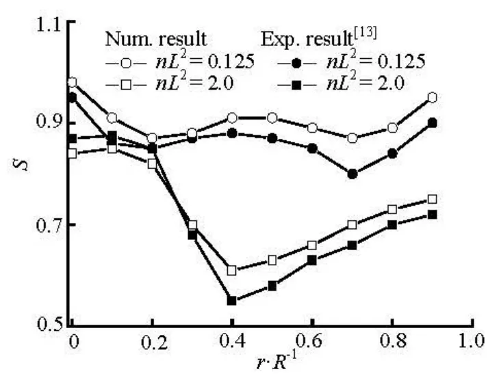
Fig.9 Distributions of orientation order parameter at x/ R =–2
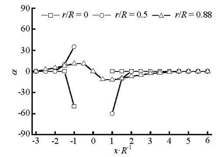
Fig.10 Preferred angles in the flow direction for the fibers with completely aligned orientation initially at inlet (a11=1, a12=0) (nL2=0.125)
4.2 Fiber orientation distributions along the flow direction
The numerical results of the preferred anglesα along the flow direction at r/ R=0, 0.5 and 0.88 are shown in Figs.10 and 11 for the dilute and concentrated regimes. The region of-1 < x/ R <1is the location of the sphere. On the centerline(r/ R =0),α for the dilute case suddenly decreases from α=0oto–50° in the region immediately upstream of the sphere, andαis zero in the downstream region of the sphere. In contrast, for concentrated caseαabruptly increases from α=0oto 88oin front of the sphere, furthermore in the immediately downstream region it increases from -75oto 10o. In the regions between the centerline and the side wall (r/ R =0.5)and near the side wall(r/ R =0.88),αrapidly returns to zero in a short distance behind the sphere(x/ R ≈2.0)for the dilute case, and in the further downstream region, αshows very little change. However, for the concentrated one,αgrows more slowly compared with those for the dilute one, and gradually returns to the flow direction in the far downstream region(x/ R≥4.0) for r/ R =0.88, whereasαreaches a plateau at x/ R ≈4.0and keeps the value around -10ofor r/ R =0.5. It demonstrates that the obstacle such as the sphere in the flow strongly disturbs the fiber orientation state in the concentrated suspension, while it gives relatively small effect on the orientation state in the dilute one.
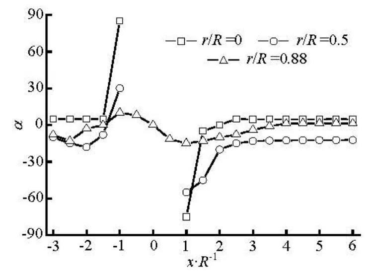
Fig.11 Preferred angles in the flow direction for the fibers with moderately orientation initially at inlet (nL2=2.0)
Fiber orientation distribution depends on the flow field and the fiber interactions including the mechanical and hydrodynamic effects. In the present study, the initial flows in all the cases are the same. Therefore, the difference of fiber orientation for the dilute and concentrated regimes is resulted from the fiber interaction. For the dilute one, the mechanical interactions between fibers are insignificant, and the centroid of fiber is generally expected to move on the streamline. In this case, the hydrodynamic interaction plays an important role on the fiber orientation distribution. However, in the concentrated one, the mechanical interactions between fibers are significant. In the region where the flow suddenly changes, e.g., immediately downstream of sphere, the fibers quickly rotate and even the slight mechanical interactions between fibers play a significant role in the fiber orientation distribution.
4.3 Effect of initial orientations at inlet
The fiber orientation distributions with different initial orientations at inlet are studied in order to explore the effect of initial conditions on the fiber orie-ntation. Here the completely aligned fibers at inlet are introduced andλis defined as the angle between the fiber axis and thex -axis.
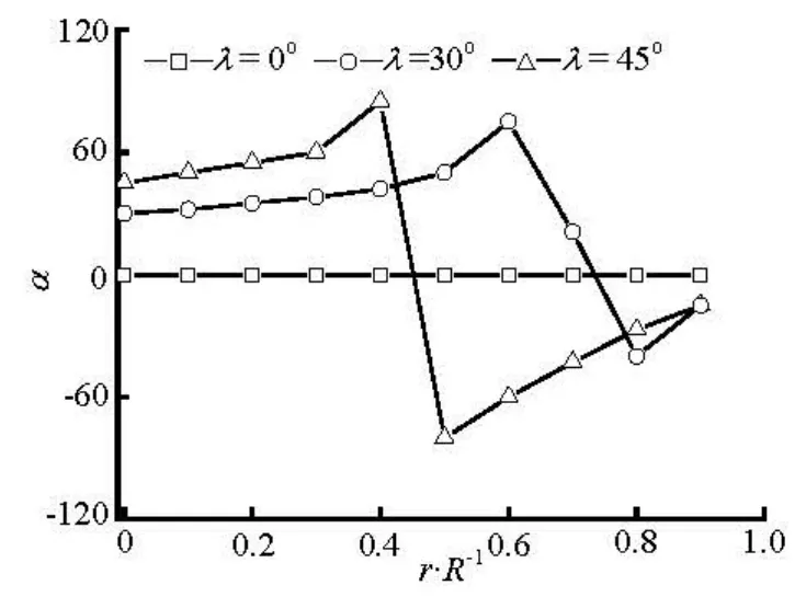
Fig.12 Preferred angles at x/ R=–2 for various initial orientation at inlet (nL2=0.125)
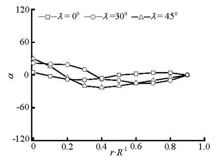
Fig.13 Preferred angles at x/ R=–2 for various initial orientation at inlet (nL2=2.0)
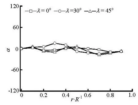
Fig.14 Preferred angles atx/ R=2 for various initial orientation at inlet (nL2=0.125)
Figures 12-15 show the transverse distributions of the preferred anglesα, in the upstream region (x/ R = -2)and the downstream region (x/ R =2) of the sphere, for the two concentration regimes with various initial orientations at inlet. As is shown in Figs.12 and 13, the fiber orientation is strongly dependent on the initial orientation at inlet in the upstream region of the sphere, and this is particularly true for the dilute suspension. Therefore, aligning the fibers at inlet along the flow direction has a beneficial effect on the fiber alignment with the flow direction in the upstream region of the sphere. However, the initial orientation angles have little effect on the fiber orientation in the downstream region(x/ R =2)of the sphere because the profiles of the preferred angles for differentλare nearly the same as shown in Figs.14 and 15.
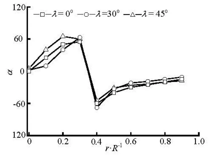
Fig.15 Preferred angles atx/ R=2 for various initial orientation at inlet (nL2=2.0)
Based on the above discussion we can conclude that the fiber orientation in the upstream of the sphere is greatly influenced by the initial orientation at inlet, while downstream of the sphere is relatively insensitive to the initial orientation because the fibers with any initial orientation at inlet will align with the flow direction when they flow through the region between the sphere and wall.
5. Conclusion
For dilute and concentrated suspensions the fiber orientation distributions have been simulated numerically with the LBM in fiber suspensions flow through a tube containing a sphere. In the simulations the interactions between fibers, fiber and sphere, fiber and tube wall are taken into account. The numerical results of orientation distribution are in agreement with the experiment performed in a channel containing a cylinder qualitatively. The results show that the existence of sphere in the tube results in a change of the fiber orientation in the downstream region of the sphere along the flow and transverse directions because of the stretching and shearing effect caused by the sphere. The effects of the sphere on the fiber orientation distribution are more significant for the concentrated suspensions than for the dilute one. The fiber orientation distribution in the upstream of the sphere is greatly influenced by the initial orientation at inlet, whereas no apparent difference in the fiber orientation in the downstream of the sphere is observed.
References
[1] YASUDA K., MORI N. and NAKAMURA K. A new visualization technique for short fibers in a slit flow of fiber suspensions[J]. International Journal of Engi- neering Science, 2002, 40(9): 1037-1052.
[2] LIN J., ZHANG W. and YU Z. Numerical research on the orientation distribution of fibers immersed in laminar and turbulent pipe flows[J]. Journal of Aerosol Science, 2004, 35(1): 63-82.
[3]SALAHUDDIN A., WU J. S. and AIDUN C. K. Numerical study of rotational diffusion in sheared semidilute fibre suspension[J]. Journal of Fluid Mechanics, 2012, 692: 153-182.
[4]NISKANEN H.,ELORANTA H. and TUOMELA J. et al. On the orientation probability distribution of flexible fibres in a contracting channel flow[J]. International Journal of Multiphase Flow, 2011, 37(4): 336-345.
[5] LIN J., SHI X. and YOU Z. Effects of the aspect ratio on the sedimentation of a fiber in Newtonian fluids[J]. Journal of Aerosol Science, 2003, 34(7): 909-921.
[6] LIN J., SHI X. and YU Z. The motion of fibers in an evolving mixing layer[J]. International Journal of Multiphase Flow, 2003, 29(8): 1355-1372.
[7]YU Z.,PHAN-THIEN N. and TANNER R. I. Rotation of a spheroid in a couette flow at moderate Reynolds numbers[J]. Physical Review E, 2007, 76(2): 026310.
[8] LADD A. J. C., COLVIN M. E. and FRENKEI D. Application of lattice-gas cellular automata to the Brownian motion of solids in suspension[J]. Physical Review Letters, 1988, 60(11): 975-978.
[9] AIDUN C. K., LU Y. and DING E. Direct analysis of particulate suspension with inertia using the discrete Boltzmann equation[J]. Journal of Fluid Mecha- nics,1998, 373: 287-311.
[10] DING E.-J., AIDUN C. K. Extension of the lattice-Boltzmann method for direct simulation of suspended particles near contact[J]. Journal of Statistical Physics, 2003, 112(3-4): 685-708.
[11]VENTURA C.,GARCIA F. and FERREIRA P. et al. Flow dynamics of pulp fiber suspensions[J]. TAPPI Journal, 2008, 7(8): 20-26.
[12]WIKLUND J. A.,STADING M. andPETTERSSON A. J. et al. A comparative study of UVP and LDA techniques for pulp suspensions in pipe flow[J]. AICHE Journal, 2006, 56(2): 484-495.
[13] YASUDA K., KYUTO T. and MORI N. An experimental study of flow-induced fiber orientation and concentration distributions in a concentrated suspension flow through a slit channel containing a cylinder[J]. Rheolo- gica Acta, 2004, 43(2): 137-145.
[14] YASUDA K., HENMI S. and MORI N. Effects of abrupt expansion geometries on flow-induced fiber orientation and concentration distributions in slit channel flows of fiber suspensions[J]. Polymer Composi- tes, 2005, 26(5): 660-670.
[15] CHEN S., DOOLEN G. D. Lattice Boltzmann method for fluid flows[J]. Annual Review Fluid Mechanics, 1998, 30: 329-364.
[16] GUO Z., ZHAO T. Explicit finite-difference lattice Boltzmann method for curvilinear coordinates[J]. Physical Review E, 2003, 67(6): 066709.
10.1016/S1001-6058(13)60352-2
* Project supported by the Doctoral Program of Higher Education in China (Grant No. 20120101110121).
Biography: LIANG Xiao-yu (1975-), Male, Ph. D. Candidate, Associate Professor

- 水动力学研究与进展 B辑的其它文章
- Hydrodynamic modeling of cochlea and numerical simulation for cochlear traveling wave with consideration of fluid-structure interaction*
- Numerical analysis of vortex core phenomenon during draining from cylinder tank for various initial swirling speeds and various tank and drain port sizes*
- Radiation and diffraction analysis of a cylindrical body with a moon pool*
- Heat transfer characteristics in micro-fin tube equipped with double twisted tapes: Effect of twisted tape and micro-fin tube arrangements*
- Stochastic simulation of fluid flow in porous media by the complex variable expression method*
- Effects of high-order nonlinearity and rotation on the fission of internal solitary waves in the South China Sea*