
Simulation and analysis of ice processes in an artificial open channel*
2013-06-01 12:29GUOXinlei郭新蕾YANGKailin杨开林FUHui付辉WANGTao王涛
水动力学研究与进展 B辑 2013年4期
关键词:王涛
GUO Xin-lei (郭新蕾), YANG Kai-lin (杨开林), FU Hui (付辉), WANG Tao (王涛),
GUO Yong-xin (郭永鑫)
State Key Laboratory of Simulation and Regulation of Water Cycle in River Basin, China Institute of Water Resources and Hydropower Research, Beijing 100038, China, E-mail: guoxinlei@163.com
Simulation and analysis of ice processes in an artificial open channel*
GUO Xin-lei (郭新蕾), YANG Kai-lin (杨开林), FU Hui (付辉), WANG Tao (王涛),
GUO Yong-xin (郭永鑫)
State Key Laboratory of Simulation and Regulation of Water Cycle in River Basin, China Institute of Water Resources and Hydropower Research, Beijing 100038, China, E-mail: guoxinlei@163.com
(Received July 17, 2012, Revised September 24, 2012)
The Middle Route Project for South-to-North Water Transfer, which consists of a long artificial open channel and various hydraulic constructions, is a big water conveyance system. A numerical modeling of water conveyance in the ice period for such large-scale and long distance water transfer project is developed based on the integration of a river ice model and an unsteady flow model with complex inner boundaries. A simplified method to obtain the same flow discharge in the upstream and downstream of the structure by neglecting the storage effect is proposed for dealing with the inner boundaries. According to the measured and design data in winter-spring period, the whole ice process, which includes the formation of the ice cover, its development, the melting and the breaking up as well as the ice-water dynamic response during the gate operation for the middle route, is simulated. The ice characteristics and the water conveyance capacity are both analyzed and thus the hydraulic control conditions for a safety regulation are obtained. At last, the uncertainties of some parameters related to the ice model are discussed.
ice process, simulation, open channel, middle route
Introduction
The Middle Route Project for South-to-North Water Transfer is regarded as the most effective way to alleviate the water shortage in North-China. The project consisting of a long artificial open channel and various hydraulic constructions plans to transfer water from the Taocha to Beijing. It spans eight degrees in latitude and the water is transferred from a temperate zone to a colder region. During winter months, the water conveyance will experience various stages including those of no ice, ice cover forming, melting and breaking up. There is a risk that the ice jam will form by accumulations of frazil ice in some gates and inverted siphons especially in the north of Anyang region. Since it is difficult to analyze the ice condition in a field test at present, the numerical modeling provides a viable alternative to better understand the processes and to provide a tool to evaluate strategies for the safety regulation.
Several river ice models were developed in past years. Lal and Shen[1]developed a model called RICE, which is based on the concept of the two-layer ice transport by considering that the ice discharge in the river consists of surface and suspended ice discharges. The model involves the water temperature and ice discharge distributions, the ice cover evolution and under cover deposition and erosion. Beltaos[2]developed a one-dimensional numerical model named RIVJAM for computing static ice jam profiles. Since the river ice transport and the jam processes are two-dimensional phenomena owing to the existence of the bank friction and the irregular channel geometry, Shen et al.[3]developed a two-dimensional DynaRICE model to simulate the ice jam dynamics. Zufelt and Ettema[4]developed a one dimensional unsteady flow model to simulate the dynamic failure and the reformation of an ice jam. Beltaos[5]reviewed studies of numerical modeling of river ice processes, and this paper will provide more detailed information of ice-jam modeling. Recently, Kandamby et al.[6]developed a model called RICE-E, based on the RICEN model, which can simulate flowand ice conditions in rivers with floodplains. Lindenschmidt et al.[7]used the ice jam model RIVICE in the lower reach of the Red River to evaluate the strategies for the ice jam mitigation. In China, Yang et al.[8]put forward a range of formulas to describe the dynamics of the ice cover, and obtained a uniform form to represent the diffusion of frazil in an open flow and an ice covered flow, the heat exchange of the ice cover and the floating ice floe,and the accumulation and erosion of frazil and ice floes. The model was verified and applied to Songhua River. Sui et al.[9]used the HEC-RAS software to simulate the flow and to determine the thickness of the ice jam, with the initial cover being given beforehand. Wang et al.[10]developed a three-dimensional model to simulate the floating rates of frazil ice particles in water under a covered condition. Mao et al.[11]presented a synthetic and dynamic mathematical model for the ice jam simulation, which was validated by the measurement data on the Hequ section of the Yellow River. Gao et al.[12]analyzed the water temperature and the relationship between the ice discharge distribution and the air temperature in the middle route project, but the model could not simulate the ice cover forming and the development process. Although the models such as RICE and RICEN are capable of describing the dynamic transport of the ice and the ice jam formation, the application of the models to such a large-scale artificial open channel with enormous hydraulic structures (e.g., turnouts, junctions, gates etc.) distributed along is still a challenge. An ice modeling system suitable for this project should be independently developed.
This paper focuses on the exploitation and application of the numerical modeling system of the ice process for the middle route open channel. The main models are based on the RICE model presented by Lal and Shen[1], further developed by Yang et al.[8,13]and coupled with the unsteady flow model with complex inner boundaries. A simplified method for inner boundaries and an artificial fluid method are used to calculate the dynamic ice cover progression[14]. With these modifications, the modeling system is applied to analyze the ice-water dynamic response during the gate operation and the whole ice process for the middle route according to the measured and design data in the winter-spring period. The ice characteristics and the water conveyance capacity are both analyzed.
1. Numerical models
1.1 Modeling of the unsteady flow in main channel
The hydraulics of a one-dimensional channel flow can be described by Saint Venant equations. For a channel with a floating ice cover, the flow resistance terms are calculated in terms of Manning’s coefficients of the channel bed and the underside of the surface ice[1]. The governing equations with considerations of the effect of the ice cover are similar to the equations for a free surface flow. The widely used implicit fourpoint finite difference scheme is used to solve the two equations.
The Saint Venant equations are applicable to channel reaches only. For the other hydraulic structures (such as gate, tunnel, inverted siphon etc.) in series connection, two other equations equivalent to the above equations are required to account for the flow through those structures. It is extremely difficult to simulate the detailed flow pattern around the structures using a one-dimensional model, so a simplified method is used, by neglecting the storage effect of the hydraulic structure, imposing the same flow discharge in the upstream and the downstream of the structure. In the method, the inner boundaries are represented as a short channel. An iteration scheme for the continuity equation and the energy equation can be derived by performing a Taylor series expansion up to the first order as follows:
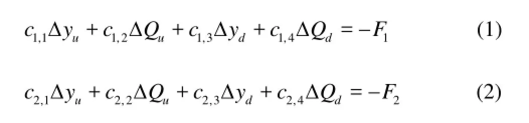
where yΔ and QΔ are the water level and discharge increments at time level +1n, subscript u and d represent the upstream and downstream nodes, respectively,1F and2F are the functions of the water level and the discharge at time level n and c1,1,c1,2,…,c2,3, c2,4are the coefficients of the two equations, computed with known values at time level n. Different types of hydraulic structures would assume different coefficients. Using an implicit four-point finite difference scheme to discretize the Saint Venant equation, Eqs.(1) and (2) can be incorporated in the solution algorithm.
1.2 Ice mathematical models
The distribution of the water temperature along a channel can be described as
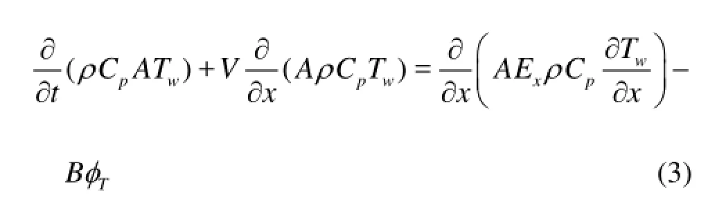
where ρ is the water density, Cpis the specific heat of water, A is the cross-sectional area of the channel, Twis the cross-section-averaged water temperature, V is the cr oss-section -averaged velocity, Exis the longitudinaldispersioncoefficient of heat, B is thechannel width,Tφ is the total heat loss rate per unit surface area of the river including the heat exchange between water and air, ice and water, water and river.
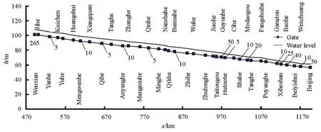
Fig.1 Basic hydraulic parameters for Wenxian-Beijing channel
When the water temperature drops below the freezing point in winter, the frazil ice will be produced. The one-dimensional advection-diffusion equation for the frail ice concentration becomes
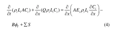
whereiC is the ice concentration,iρ is the ice density, Liis the latent heat of fusion of water, ΣS is the additional source or sink terms due to the ice cover progression, erosion, deposition and melting.
If the air temperature is kept below the freezing point for some time, the thickness and the surface area of the floating ice will increase along with a downstream movement. The surface ice area concentration can be written as
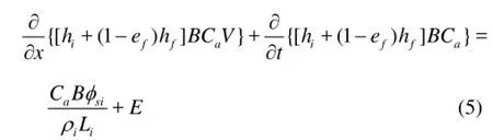
whereaC is the area concentration, or the fraction of the water surface area covered by floating ice particles, ih is the solid ice thickness in the floating ice pans, hfis the thickness of the frazil ice on the underside of floating ice pans,fe is the porosity of the frazil ice in the surface layer,siφ is the net rate of heat loss per unit area over the portion of the water surface covered by ice, E is the net exchanges of the ice flux at the interface between the surface and the suspended layers.
The ice cover can be divided into the solid ice cover and the frazil ice cover. The thickness of the solid ice cover is mainly affected by the heat exchange, for the frazil ice cover, the thickness change is a function of the buoyancy of the frazil ice, the water erosion, and the growth of the solid ice cover. The rate of the growth of the solid ice thickness can be calculated as
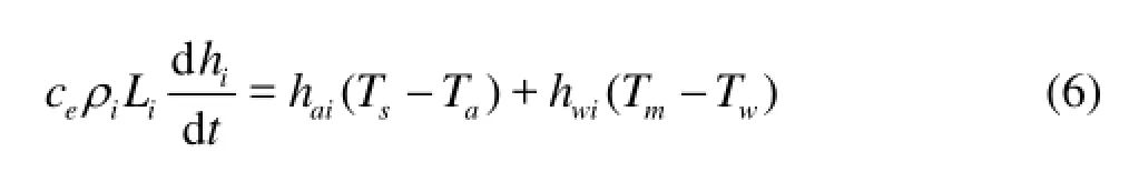
whereec is the porosity of the solid ice layer with consideration of the accumulation of the frazil ice,aih is the heat exchange coefficient between air and ice, Tsis the temperature at the ice surface, Tais the air temperature,wih is the heat exchange coefficient between water and ice andmT is the freezing point of ice.
The rate of growth of the frazil ice thickness can be deduced as
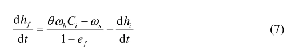
wheresω is the rate of the frazil ice erosion.
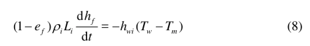
The decrease rate of the frazil ice thickness can be described as
Along with the ice accumulation and the downstream transport, the progression of the ice cover is a dynamic process and its rate can be calculated as
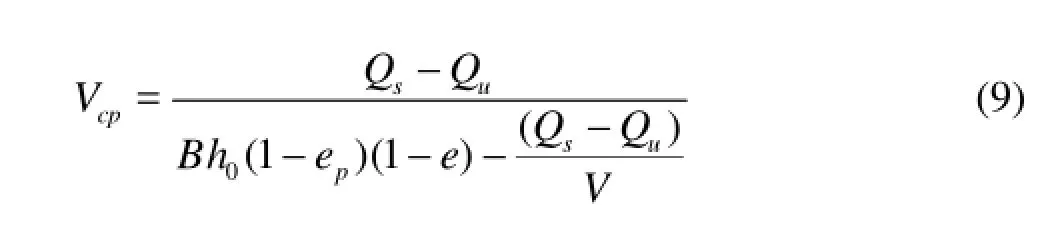
wherecpV is the rate of progression of the leading edge, 0h is the initial cover thickness, pe is the porosity in the accumulation representing the voids between floes, e is the porosity of individual ice floes, Qsis the surface ice discharge, Quis the volumetric rate of the ice entrainment under the cover at the leading edge.
Since the details of the computation methods can be found in Ref.[1], they will not be repeated here. The artificial fluid method developed to calculate the dynamic ice cover progression was presented by Fu et al.[14]. The modeling system was validated with analytical and numerical solutions for an idealized case constructed by Lal and Shen[1]. Two solutions give comparable results.
2. Application
The open channel considered in this research is a segment from Wenxian County(jumping-off point of the Yellow River) to Beijing with a total length of 703.2 km (The start and stop stake numbers are 493+ 138 and 1 196+362, respectively), as shown in Fig.1. A total of 35 gates, 67 inverted siphons, 15 main turnouts, 11 culverts and 11 flumes etc. are distributed along the channel. The channel is separated into 78 computational “pools” by the above hydraulic structures and ice booms. The water discharge of each pool and the turnout along the channel are also given. The model parameters such as the bed roughness coefficients and the stage-discharge relationship of various hydraulic structures were calibrated first under the open water condition. Because the project is not yet in a full operation, the parameters related to the ice process (the critical Froude numbers, the ice cover roughness coefficients, the buoyant velocity, the ice cover porosity and cohesion, etc.) could not be calibrated by observations. Adjustments of these parameters at each stage are carried out based on the field observation data of other rivers or channels in northern China and the proposed values in Ref.[1].
The design purpose of the main channel in winter is firstly to form a stable ice cover in each pool as soon as possible, then to increase the flow rate under the ice cover to meet the water allocation requirements along the channel. A critical Froude number or velocity has long been accepted as a means of determining the ice formation mode. For the particle juxtaposition model, Fr≤0.055 is used in this study as the control condition during the open water in terms of the safety regulation. Thus, the initial condition is a steady state open water flow with 25% of the designed discharge.
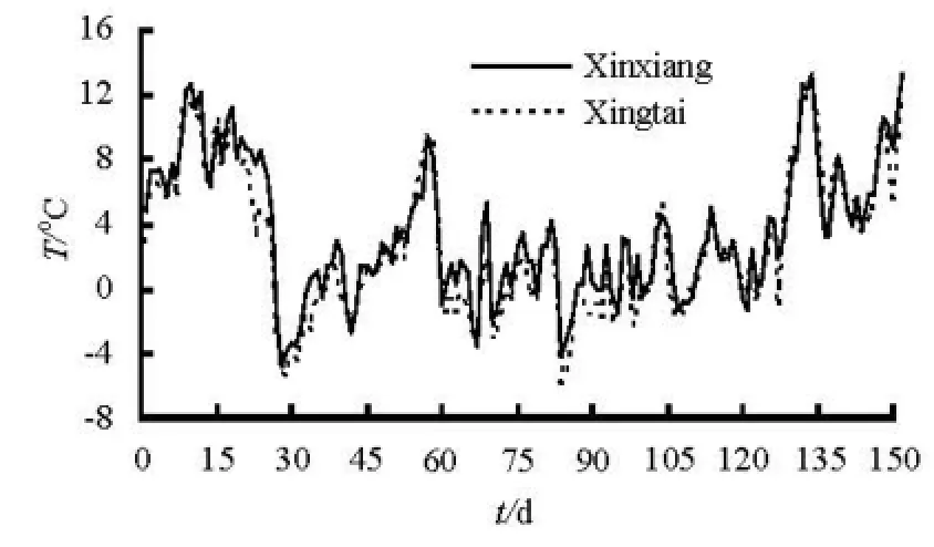
Fig.2 Variation of air temperature with time at three regions in normal winter
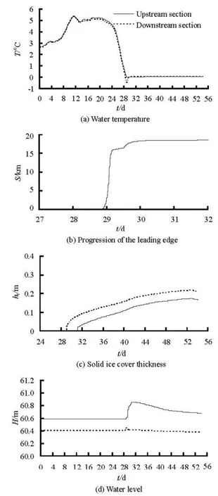
Fig.3 Variations of important flow and ice variables
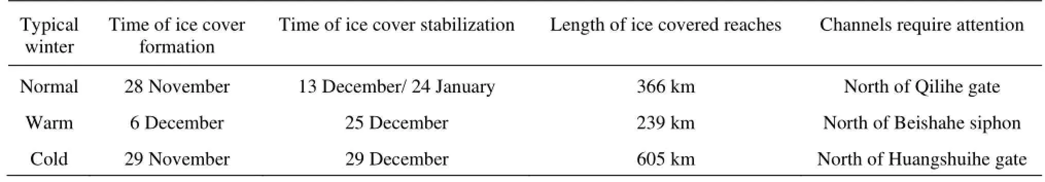
Table 1 Characteristics of ice conditions in three typical years
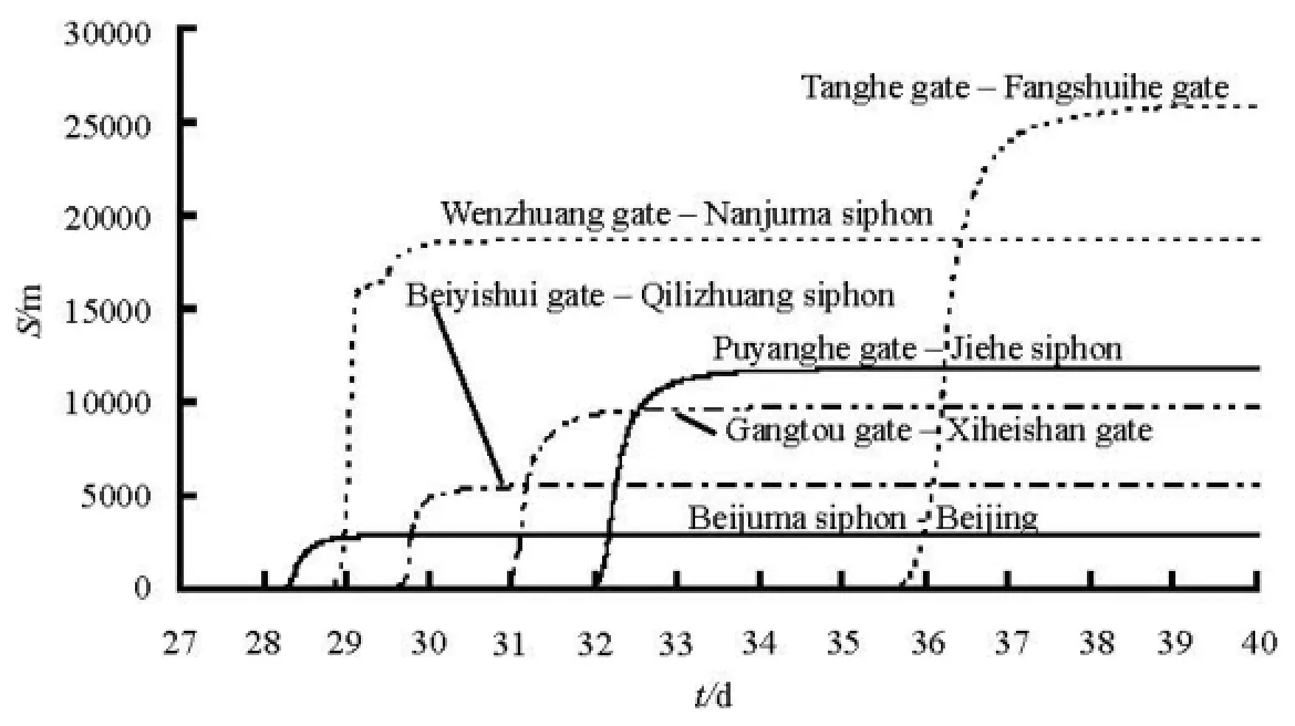
Fig.4 Evolution and progression of ice cover in each pool during the first cool-down process
Simulation runs are for about 150 d. The selected starting date is 1 November to allow the open water conditions to prevail for a few weeks before an ice cover formed and the stopping date is 30 March the following year to allow the open water conditions to prevail again after the break up. Three typical years, 1967 for cold winter, 2001 for warm winter and 1987 for normal winter, are considered for the input air temperature distribution along the channel. 2 min is used as the time step and the whole channel is divided into 1 585 calculation sections in the program. Upstream boundary conditions include a constant water discharge of 66.25 m3/s and a water temperature variation with time based on the local average daily temperature during recent 50 years. The downstream boundary condition imposed at Beijing is a water depth of 3.8 m. The initial ice cover roughness coefficient ni,i=0.03 and the heat exchange coefficient between air and ice hai=10. The variation of the air temperature with time at two representative regions from 1987 to 1988 is given in Fig.2. There is a cool-down process in late November 1987 and a rapid rise of the air temperature after that. The secondary obvious cooling process occurs in late December. The air temperature is fluctuated around zero until early March next year.
Take the channel from Wenzhuang gate to Nanjuma inverted siphon (near Beijing) as an example to demonstrate the simulated ice process in normal winter. Two sections, the section after the gate upstream and the section before the inlet of the siphon downstream, are described in detail. The time-dependent variations of the important flow and ice variables are shown in Fig.3. The water temperature declines gradually as the air temperature decreases. The water temperature goes to zero in 29 November. The frazil ice particles grow both in size and number due to the continuous surface heat loss. When the ice load becomes excessive, plenty of frazil ice particles rise to the surface and are accumulated at the downstream floating ice boom, then a skim ice cover is formed and developed. Once the water surface is covered, the heat exchange between water and air is interrupted, the water temperature under the ice cover rises to zero, as shown in Fig.3(a). As the Froude number at the leading edge is below 0.055, the ice cover develops by the juxtaposition mode at the beginning time. The inflexion on the curve in Fig.3(b) represents the change of the ice cover formation mode, which turns to the hydraulic thickening mode because the calculated Froude number at that time is between 0.055 and 0.086, which slows the formation growth. The simulation results indicate that the maximum ice thickness at the downstream section is larger than that in the upstream section. The ice accumulation reduces the upstream water discharge and increases the water levels due to the change of the wetted perimeter and the roughness. The water discharge is reduced by 27% and the maximum inc rement of t he wa ter leve l at the upstreamis0.25m.Sincethebasictrendsofthevariations of the important ice and flow variables in other pools upstream are the same as this pool, they will not be repeated here. Figure 4 shows the evolution of the ice cover under controlled hydraulic conditions. It indicates that the progression of the leading edge varies with each pool. As the air and water temperature decreases from south to north, the starting time of the ice cover to be formed in near pools is different but the possible occurrence is in 1 d. Once the ice cover developes from the beginning of the ice boom downstream in one pool, the time needed in this pool is below 2 d. It indicates that the ice cover in a near pool progresses to the upstream at the same time. That is to say, the chain of the open water–the ice covered surface–the open water–the ice covered surface can be formed during the ice forming and development process, but the development velocity and the ice thickness against time as well as against the length of the ice covered surface in each pool are different. The results for the characteristics of ice conditions are presented in Table 1. The simulated results indicate that the progression of the ice cover is in a particle juxtaposition mode at most of the time and the fluctuation of the water level is in the permitted range of the standard value under a such low controlled water discharge in all three typical years.
The above simulation results show that the safety water conveyance under the ice cover could be assured by reducing the water discharge along the main channel. After that it is time to increase the discharge and maintain these conditions until the breakup period in spring to compensate the insufficiency of the flow rate in winter. Take the cold winter as the air temperature condition, Fig.5 shows the variation of the water level in two typical sections in the whole winter. It indicates that the rational discharge under the stable ice cover should not exceed 50% of the designed flow rate due to the constraints of the maximum fluctuation of the water level. When the water discharge for the ice breakup is decreased to 25% of the designed flow rate, the effect of ice on the magnitude of resulting waves is not significant.

Fig.5 Variation of water level with time during the whole winter under controlled conditions
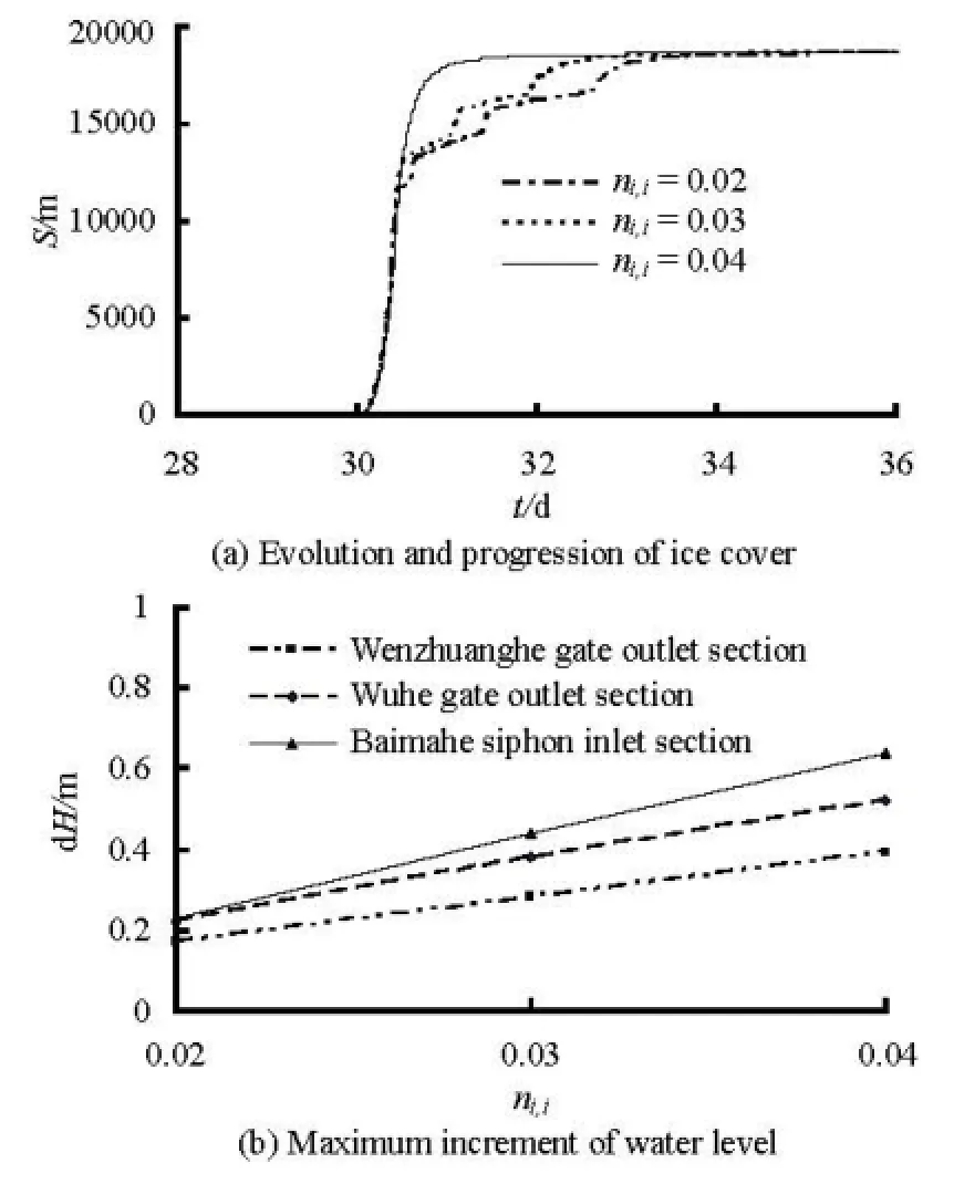
Fig.6 Influence of various,iin on the simulation of ice process
3. Uncertainties of some parameters
3.1 uncertainty of the initial ice cover roughness coefficient
The Manning’s roughness coefficient of the ice cover can be described by the following exponential function

where,ien is the roughness coefficient at the end ofthe ice covered period, which is approximately equal to that of the smooth ice cover, 0.008-0.015, k is a decay constant and t is the number of days from the beginning of the ice covered period. The initial ice cover roughness coefficient,iin is difficult to determine for a river reach with large variations in the initial ice cover thickness. Based on the observation data of other rivers, this value is between 0.02 and 0.04. Figure 6 shows the influence of various,iin on the simulation of the ice process under cold winter conditions. It indicates that the progression of the leading edge varies with the value. The effect of the water resistance would be significant when,iin is bigger, thus the water level increasing is remarkable, as shown in Fig.6(b). Due to the water level increase, the Froude number is decreased. The ice cover development process changes from the hydraulic thickening mode to the juxtaposition mode, but the starting time of the ice cover forming is not affected.
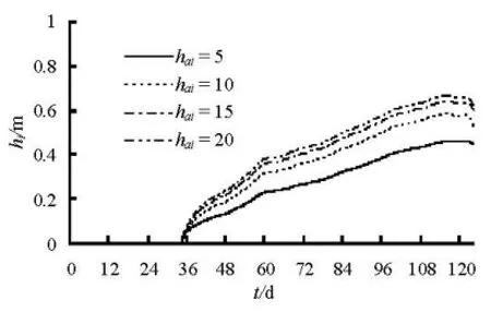
Fig.7 Solid ice cover thickness of Fangshuihe gate inlet section
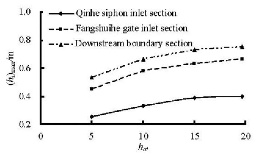
Fig.8 Influence of variousaih on the maximum solid ice cover thickness
3.2 Uncertainty ofaih
The heat exchange at the top and bottom surfaces of an ice cover governs the rate of change of the ice cover thickness. Because the frazil ice thickness is very small due to the low ice concentration after the ice cover formation, here only the solid ice thickness is considered. The uncertainty ofaih is affected by many factors, such as latitude, wind velocity, cloud cover and relative humidity. Figures 7 and 8 show the influence of variousaih on the solid ice cover thickness under cold winter conditions. It can be seen that the maximum solid ice cover thickness increases as haiincreases, which indicates that the simulated solid ice cover thickness in the application in the middle route project may be related withaih value. Thus, in view of the currently limited understanding of the ice processes, further observations should be carried out to calibrated these parameters.
4. Summary and conclusion
A numerical modeling system of the water conveyance in the ice period for a large scale artificial open channel is developed and presented. The numerical model is validated and used to study the strategies for the safety regulation in the middle route of the south-to-north water transfer project. The whole ice processes under the controlling index, which include the ice cover forming, the development, the melting and the break up during the gate operation for the project in warm, normal and cold winters are simulated. The characteristics of the ice conditions including the time of the ice cover formation, the stabilization and the length of ice covered reaches as well as the channels are obtained. The desired flow rate during the dispatching and the ice breakup periods is analyzed for the safety regulation.
However, there are some uncertainties in the application of the model. The parameters related to the ice cover, thickness and the key hydraulic controlled conditions should be firstly calibrated. It is necessary to perform some field observations in this project.
[1] LAL A. M. W., SHEN H. T. Mathematical model for river ice processes[J]. Journal of Hydraulic Engineering, ASCE, 1991, 117(7): 851-867.
[2] BELTAOS S. Numerical computation of river ice jams[J]. Canadian Journal of Civil Engineering, 1993, 20(1): 88-89.
[3] SHEN H. T., SU J. and LIU L. W. SPH simulation of river ice dynamics[J]. Journal of Computational Physics, 2000, 165(2): 752-771.
[4] ZUFELT J. E., ETTEMA R. Fully coupled model of ice-jam dynamics[J]. Journal of Cold Regions Engineering, ASCE, 2000, 14(1): 24-41.
[5] BELTAOS S. Progress in the study and management of river ice jams[J]. Cold Regions Science and Technology, 2008, 51(1): 2-19.
[6] KANDAMBY A., JAYASUNDARA N. and SHEN H. T. A numerical river ice model for Elbe River[C]. 20th IAHR International Symposium on Ice. Lahti, Finland, 2010.
[7] LINDENSCHMIDT K. E, SYDOR M. and CARSON R. et al. Ice jam modelling of the lower Red River[J]. Journal of Water Resource and Protection, 2012, 4: 1-11.
[8] YANG Kai-lin, LIU Zhi-ping and LI Gui-fen et al. Simulation of ice jam in river channels[J]. Water Resources and Hydropower Engineering, 2002, 33(10): 40-47(in Chinese).
[9] SUI Jue-yi, KARNEY Btyan W. and FENG Da-xian. Ice jams in a small river and the HEC-RAS modeling[J]. Journal of Hydrodynamics, Ser. B, 2005, 17(2): 127-133.
[10] WANG Jun, LI Qing-gang and SUI Jue-yi. Floating rate of frazil ice particles in flowing water in bend channels–a three dimensional numerical analysis[J]. Journal of Hydrodynamics, 2010, 17(2): 127-133.
[11] MAO Ze-yu, WU Jian-jiang and ZHANG Lei et al. Numerical simulation of river ice jam[J]. Advances in Water Science, 2003, 14(6): 700-705(in Chinese).
[12] GAO Pei-sheng, JIN Guo-hou and LU Bin-xiu. Preliminary study on ice regime in the middle route of south to north water transfer project[J]. Journal of Hydraulic Engineering, 2003, 34(11): 96-101(in Chinese).
[13] YANG Kai-Lin, WANG Tao and GUO Xin-lei et al. Safety regulations of water conveyance in the middle route of south-to-north water diversion project in ice period[J]. South-to-North Water Diversion and Water Science and Technology, 2011, 9(2): 1-8(in Chinese).
[14] FU Hui, YANG Kai-lin and GUO Xin-lei et al. Fictitious method for numerical simulation of cannal ice processes[J]. South-to-North Water Diversion and Water Science and Technology, 2010, 8(4): 7-12(in Chinese).
10.1016/S1001-6058(11)60394-7
* Project supported by the National Key Basic Research Program of China (973 Program, Grant No. 2013CB036405), the National Natural Science Foundation of China (Grant Nos. 51109230, 51209233).
Biography: GUO Xin-lei (1980-), Male, Ph. D., Senior Engineer
猜你喜欢
Chinese Physics B(2023年1期)2023-02-20
理科爱好者(教育教学版)(2022年2期)2022-05-05
Plasma Science and Technology(2022年2期)2022-03-10
大众文艺(2020年23期)2021-01-04
大众文艺(2020年22期)2020-12-13
艺术家(2018年12期)2018-03-18
水动力学研究与进展 B辑(2017年1期)2017-03-09

- 水动力学研究与进展 B辑的其它文章
- Ship bow waves*
- Progress in numerical simulation of cavitating water jets*
- Three-dimensional large eddy simulation and vorticity analysis of unsteady cavitating flow around a twisted hydrofoil*
- Numerical simulation of shallow-water flooding using a two-dimensional finite volume model*
- Dynamical analysis of high-pressure supercritical carbon dioxide jet in well drilling*
- Micropaticle transport and deposition from electrokinetic microflow in a 90obend*