Comparison of Four Multiscale Methods for Elliptic Problems

Y.T.Wu,Y.F.Nieand Z.H.Yang

1　Introduction

In recent years many works have concentrated on simulation of complex systems composed of heterogeneous materials or media[Yang,Yu,Ryu,Cho,Kyoung,Han,and Cho(2013);Hou and Efendiev(2009);Geers,Kouznetsova,and Brekelmans(2010);Hughes and Sangalli(2007)].For example,the thermo–mechanical behavior of composite materials and flows in porous media are frequently investigated.These problems contain at least two spatial scales:one is the macroscale of structures and the other is the microscale of heterogeneities.Though classical numerical methods such as finite element method(FEM)could be used directly to simulate these multiscale problems,a main issue is that sufficiently large discrete systems should be solved which demand a tremendous amount of computer memory and CPU time.On the other hand,it is not necessary to obtain full details of the multiscale solution within the entire domain in some cases[E,Engquist,Li,Ren,and Vanden-Eijnden(2007);Zohdi and Wriggers(2005)].Therefore some multiscale methods have been developed to serve different purposes and to solve the multiscale problems efficiently in the last few decades.In this paper,four representative multiscale methods are compared and their differences and similarities are shown through analytical and numerical results,in order to help the reader have a good choice of multiscale methods for solving multiscale problems for special purpose.

The first multiscale method is the asymptotic homogenization method(AHM)which was proposed in 1970s to solve two–scale problems for periodic structures[Bensoussan,Lions,and Papanicolaou(1978);Oleinik,Shamaev,and Yosifian(1992)].AHM constructs a formal asymptotic expansion for solution of multiscale problem and provides the manner to compute zeroth–order, first–order and higher–order expanded terms.With the exception of the zeroth–order term,other terms are the combinations of microscopic functions and macroscopic functions to connect different scales.The different scales are connected further by solving auxiliary problems at the microscale to get effective coefficients of the homogenized problem defined at the macroscale[Cioranescu and Donato(1999)].For structures made up of random heterogeneous materials,Papanicolaou et al.[Papanicolaou and Varadhan(1981)]extended AHM to random case with stationarity and ergodicity assumptions on multiscale coefficients.Considering the first–order homogenization provides microscopic fields with very low accuracy,Cui et al.[Han,Cui,and Yu(2010);Yu,Cui,and Han(2009)]extended AHM to second–order and proposed a statistical second–order two–scale method.AHM has been widely used to predict thermal,electrical and mechanical properties of heterogeneous materials[Ma and Cui(2013);Arabnejad and Pasini(2013);Chatzigeorgiou,Efendiev,Charalambakis,and Lagoudas(2012)].

Heterogeneous multiscale method(HMM)gives another kind of general framework for designing multiscale methods,and a finite element formulation is proposed for elliptic homogenization problem in[E and Engquist(2003)].In general,HMM consists of two components:selecting a macroscopic solver and estimating the missing data in the solver from microscopic information.Scale separation such as periodicity and stationary randomness of the multiscale coefficients is the main special feature which HMM assumes.Diffusion problems,advection–diffusion problems,Richards’equation,etc.have been considered by HMM[Ma and Z-abaras(2011);Abdulle and Schwab(2005);Henning and Ohlberger(2010);Chen and Ren(2008)].E et al.[E,Engquist,Li,Ren,and Vanden-Eijnden(2007)]reviewed the fundamental principles,theoretical analysis and some applications of HMM and also some obstacles that need to be solved.

Variational multiscale(VMS)method was proposed by Hughes et al.[Hughes(1995);Hughes,Feijoo,Mazzei,and Quincy(1998)]to deal with multiscale problems in science and engineering.VMS method considers an overlapping sum decomposition of multiscale solution.One component of the decomposition is a sufficiently smooth function at the macroscale,and the other one is a rapidly oscillating function.The microscopic oscillating solution is localized to macroscopic elements and is semi–solved first,and then the macroscopic solution is solved when the microscopic solution is substituted into the macroscopic problem.VMS method has been used to simulate turbulent channel flows,laminar and turbulent flows,etc.[Hughes,Oberai,and Mazzei(2001);Hughes,Mazzei,Oberai,and Wray(2001);Gravemeier(2006)].Stochastic variational multiscale method has also been proposed for multiscale problems with random heterogeneities[Asokan and Zabaras(2006);Zabaras and Ganapathysubramanian(2009)].

Hou et al.[Hou and Wu(1997);Hou,Wu,and Cai(1999)]proposed the multiscale finite element method(MsFEM)for solving multiscale problems.The main idea of MsFEM is to construct special finite element base functions,which capture the microscopic information,in the macroscopic mesh.Unlike classical smooth polynomial base functions,these base functions are oscillatory functions which reflect the effect of microscale on the macroscale.MsFEM has been applied for many multiscale problems such as groundwater flow[Ye,Xue,and Xie(2004);He and Ren(2006)],two–phase flow[Efendiev,Ginting,Hou,and Ewing(2006);Efendiev and Hou(2007)]and(un)saturated water flows[He and Ren(2009);Zhang,Fu,and Wu(2009)]in heterogeneous porous media.An extended multiscale finite element method was developed by Zhang et al.[Zhang,Wu,and Fu(2010a,b)]for solving mechanical problems of heterogeneous materials.Additional terms of base functions for the interpolation of the vector fields were introduced in their works.

Apart from multiscale methods,some homogenization methods have been developed to predict effective properties of heterogeneous materials or media,see[Ma,Temizer,and Wriggers(2011);Sab and Nedjar(2005);Wang and Pan(2008)]and references therein.Recently,Dong et al.developed a novel method termed Computational Grains for predicting effective properties of heterogeneous materials with arbitrary–shaped inclusions and voids[Dong and Atluri(2012a,b);Dong,Gamal,and Atluri(2013)].The method is efficient because no meshing is required in each grain which contains a inclusion or a void and then the computational cost can be reduced.With the effective properties at hand,one can solve the macroscopic solutions of the multiscale problems conveniently.

The remainder of this paper is organized as follows.An overview of the four multiscale methods is presented in section 2.In section 3 we analyze the differences and similarities of these methods and compare their computational cost.AHM and HMM in resolving multiscale solution in local domains is compared further in this section.A numerical example to illustrate the application of these methods to random heterogeneous materials is given in section 4.And conclusions are drawn in the last section.

2　Multiscale methods

We consider the classical second–order elliptic problem with homogeneous Dirichlet boundary condition

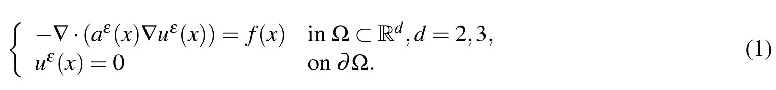
This problem is widely applied in practical problems such as thermal or electrical conductivity,mechanical properties of composite materials and flows in porous media.The coefficients in this problem possess multiscale characteristic,which is described by a parameterε.The source termfis a macroscopic function however.

We assume thatis symmetric and satisfies

with 0＜c≤C,such that the problem has a unique solutionuεfor anyε[Braess(2001)].To get an accurate numerical solution,a full fine scale solver such as fine FEM with meshThcannot be avoided.The mesh sizehcannot be larger than the size of heterogeneities in order to offer some details of the multiscale solution.The fact leads to a big challenge of solving an extremely large discrete system,which is the reason why the following multiscale methods were proposed to obtain an approximation of the multiscale solutionuε.

2.1　Asymptotic homogenization method

The macroscopic behavior of heterogeneous material may be approximated by that of a homogeneous fictitious one,when the characteristic length of the heterogeneities is sufficiently small compared to the characteristic length of the structure.Asymptotic homogenization method(AHM)shows that under some assumptions on the multiscale coefficientsaε,there exists a homogenized problem defined at the macroscale such that solution of the original multiscale problem converges to solution of the homogenized problem as the small parameterεgoes to zero.As a consequence,AHM first estimates the macroscopic behavior of the heterogeneous material by solving a macroscopic problem which could significantly reduce the amount of computation.

It is assumed that the multiscale coefficientsaεtake the formfor simplicity.In this caseaεmay be a periodic function or a stationary random function de fined in the entire domain,which can be used to describe a lot of heterogeneous materials.AHM provides a formal asymptotic expansion of the multiscale solution

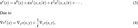
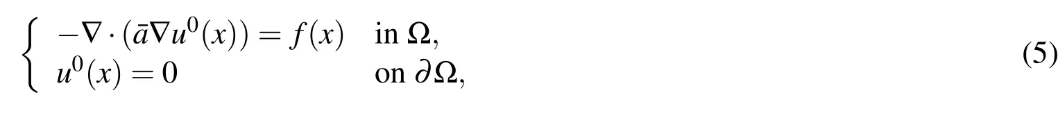
wherewhen we insert Eq.3 into the multiscale problem(Eq.1)and equate coefficients of the same powers ofε,it is found thatu0is the solution of a homogenized problem

HereYis an arbitrary domain at the microscale,andλin the Dirichlet boundary condition is a constant vector.It should be noted that other boundary conditions such as periodic boundary condition or Neumann boundary condition can be employed instead of Dirichlet boundary condition,see[Kanit,Forest,Galliet,Mounoury,and Jeulin(2003);Yue and E(2007)]for more details.A repeated unit cell(RUC)is used to compute effective coefficients for periodic structures.In contrast,for random heterogeneous materials,a representative volume element(RVE)is always used.A schematic diagram of RUC and RVE is presented in Fig.1.

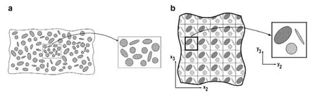
Figure 1:Description of RVE(a)and RUC(b)[Pindera,Khatam,Drago,and Bansal(2009)]

A non–rigorous definition of RVE is that it is a subdomain of random heterogeneous materials which is large enough so that the resulting effective coefficients have little dependence on the boundary condition applied in the auxiliary problems.It is expected that the characteristic length of RVE is much larger than that of heterogeneities but much smaller than that of macroscopic structures.In fact,theoretically the effective coefficients are defined in abstract probability spaces and cannot be explicitly obtained.According to the ergodic theory,the effective coefficients could be computed by solving auxiliary limit problems in the in finite physical space.This is the foundation of computing the effective coefficients in finite RVEs applied in many engineering problems.Note that the RVEs only provide approximations of the effective coefficients for random heterogeneous materials,and the accuracy of the approximations depends strongly on the size of RVEs and the boundary condition employed,see[Wu,Nie,and Yang(2014)]for detailed discussions.

when the auxiliary problems(Eq.6)are solved.Hereh·imeans the volume average of the variables in

In some cases the macroscopic behavior is enough and it is not necessary to resolve all the details of the multiscale problem.AHM solves some microscopic auxiliary problems and a macroscopic homogenized problem numerically.Compared with the fine FEM,the amount of computation is extremely reduced.However,sometimes the multiscale solution should be resolved in some local domains or in the global domain.To this end,AHM provides a strategy to resolve the multiscale solution taking advantage of the formal asymptotic expansion,that is,

whereare the canonical bases inThe first–order AHM approximates the multiscale solutionuεby the first–order solutionwhich includes additional microscopic information introduced by the microscopic functionsχei.To improve the accuracy of the multiscale solution given by AHM,higher–order AHM has also been considered,see Cui et al.[Yang,Cui,Nie,and Ma(2012);Yang and Cui(2013)],Xiao et al.[Xiao and Karihaloo(2010)]and references therein.In fact,for periodic structures,the multiscale solution in the global domain is explicitly obtained when both the auxiliary problems and the homogenized problem are solved.However for random heterogeneous materials,additional work should be done to solve the auxiliary problems in some local domains which we are interested in or in the global domain to obtain the multiscale solution.

2.2　Heterogeneous multiscale method

G–convergence[Zhikov,Kozlov,and Oleinik(1994)]in homogenization theory shows that for a sequence of multiscale coefficientsaε,ε＞0 satisfying Eq.2 for anyε,the solutionuεof the multiscale problem(Eq.1)converges to the solution of the homogenized problem(Eq.5)asεgoes to zero.Based on this fact,the heterogeneous multiscale method(HMM)solves the homogenized problem by choosing a macroscopic solver such as the coarse FEM.It is assumed thatis the standard piecewise linear finite element space on a macroscopic meshwith sizeH.Then the discrete variational formulation of the homogenized problem is:Findsuch that

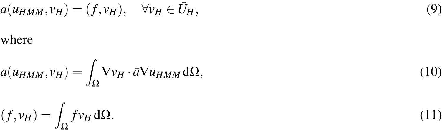
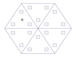
Figure 2:Illustration of HMM[E,Ming,and Zhang(2005)]

wherexkandωkare the macroscopic quadrature points and weights in elementK,andnKis the number of nodes inK.To couple the microscale and the macroscale,the following microscopic problems

are solved around any quadrature pointxkand for any base functionHereI(xk)is a small cube centered atxk.It may be an RUC for periodic structures or an RVE for random heterogeneous materials in thexcoordinates.Then the integrand atxkin Eq.12 is approximated by

When the effective stiffness matrix is computed,the variational problem(Eq.9)is solved finally to get the HMM solutionuHMMwhich is an approximation of the homogenized solutionu0.In fact,HMM estimates the effective integrands in Eq.12,but AHM directly estimates the effective coefficients¯ain Eq.12 by solving auxiliary problems(Eq.6)locally around every quadrature pointxkand then computing Eq.7.

HMM assumes that the multiscale problem(Eq.1)satis fies separation of scales.That is,characteristic length of the microscaleO(l)is much smaller than characteristic length of the macroscaleO(1),and then there exist RUCs or RVEs of sizeδsuch thatl?δ?1.With scale separation assumption,HMM simply solves some microscopic problems(Eq.13)and a macroscopic problem(Eq.9)to capture the macroscopic behavior of the multiscale problem.Therefore its computational cost is much less than that of fine FEM.

To recover the details of the multiscale solution in some local domains,HMM adopts a strategy proposed by Oden et al.[Oden and Vemaganti(2000)].After the homogenized problem is solved,the following problem

is solved with fine meshto obtain the multiscale solutionin a local domainΩL.The HMM solutionuHMMacts as a known Dirichlet boundary condition on the boundary of ΩL.We should note that though a more accurate approximationof original multiscale solutionuεin Eq.1 can be obtained,the characteristic length of ΩLshould be much smaller than the characteristic length of Ω considering the limit of capability of computing resources,but should be much larger than the characteristic length of heterogeneities because the boundary condition has great effect on the accuracy ofwhen ΩLis very small.In computation,the size of ΩLmay be very close to the RVE(RUC)sizeδ.

2.3　Variational multiscale method

The variational multiscale(VMS)method assumes that solution of the multiscale problem(Eq.1)can be decomposed into two parts,namelywhere¯urepresents a smooth function andu0a rapidly oscillating function,as shown in Fig.3.Therefore the variational formulation of Eq.1 needs to be decomposed into a macroscopic variational formulation and a microscopic variational formulation.VMS method semi–solves the microscopic variational problem first to get an expression of microscopic solutionu0,and then substitutes it into the macroscopic variational problem to solve the macroscopic solution¯u.

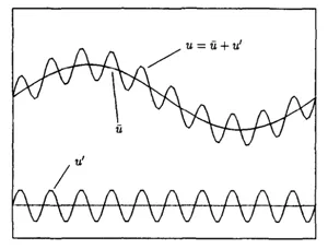
Figure 3:An overlapping sum decomposition of multiscale solution[Hughes,Feijoo,Mazzei,and Quincy(1998)]

Specifically,the variational formulation of Eq.1 is:Findsuch that

The left–hand side and the right–hand side of the equation are de fined similar to Eq.10 and Eq.11,respectively.This equation can be rewritten as

Here the solution spaceXis decomposed aswhereis the solution space for the macroscale andX0is the solution space for the microscale.Eq.18 and Eq.19 are the macroscopic variational formulation and microscopic variational formulation respectively.Thoughu0is a nonlocal function,we can only estimate it locally at the microscale.Assuming thatu0equals to zero on the boundaries of the macroscopic meshfor solving¯u,VMS method suggests to introduce residual–free bubbles which are de fined in every macroscopic elementin order to computeu0locally.Since¯uin the elementKcan be expressed as

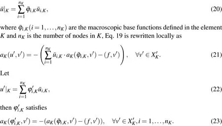
Hereare the residual–free bubbles which are zero on element boundaryE-q.23 in every macroscopic element are solved first to obtain all of the residual–free bubbles,and then the macroscopic solution can be resolved by solving the macroscopic variational problem(Eq.18)with meshtaking advantage of Eq.22.It should be mentioned that since the microscopic solution is constructed by the linear combination of residual–free bubbles with macroscopic solution at the nodes as the coefficients,the multiscale solution has been obtained by VMS method.

2.4　Multiscale finite element method

The main idea of the multiscale finite element method(MsFEM)is to construct special finite element base functions at the macroscale which can capture the microscopic information.These base functions are obtained by solving some problems in every macroscopic element.And then a small discrete system is solved at the macroscale to get the macroscopic solution.

To solve the multiscale problem(Eq.1),the domain is partitioned first into macroscopic finite elements(see Fig.4).Letwhereare the linear base functions de fined in the elementandnKis the number of nodes inK.It is a common knowledge that the standard piecewise linear if nite element spacecannot resolve all the features of the multiscale solution.MsFEM solves the following problems

to construct special multiscale base functionsfor everyKand 1≤i≤nK.Compared with linear functions,theseare oscillatory functions in every element but share the same trace with.When Eq.24 are numerically solved with meshin every macroscopic element(see microscopic mesh in Fig.4),an approximate solution of the multiscale problem(Eq.1)is found inthe special multiscale solution spacewhere Though only the approximate values of the multiscale solution at every macroscopic node are obtained,can givean approximation of multiscale solution due to the fact that the base functions have captured the microscopic information.

Figure 4:Macroscopic mesh and microscopic meshes in MsFEM[Hou and E-fendiev(2009)]

3　Comparison of the four multiscale methods

3.1　Two frameworks

Since the characteristic length of microscale is much smaller than the characteristic length of macroscale,it is impossible to find high–precision numerical solutions for multiscale problems by the fine FEM in practice.Therefore approximations of the multiscale solutions should be considered by designing effective multiscale methods.The four methods recalled in the above section can be divided broadly into two categories.AHM and HMM belong to the up–down framework,while VMS method and MsFEM belong to the uncoupling framework.

As can be seen in Fig.5,based on the homogenization theory,the up–down framework focuses first on the macroscopic behavior of the multiscale problem.The homogenized problem is considered to be solved with macroscopic mesh.Since the effective coefficients are unknown a priori,one needs to solve some auxiliary problems in some local domains at the microscale(e.g.,around quadrature points in macroscopic elements),and then to compute effective information for solution of homogenized problem.Since the microscopic auxiliary problems in different local domains are independent problems,these problems can be solved effectively by parallel computing.The number of auxiliary problems depends on the special feature of the multiscale problem.If the feature of the multiscale coefficients is uniform in the global domain,the effective coefficients are uniform and the auxiliary problems could be solved in any local domain.Otherwise,the effective coefficients depend on the macroscopic positions and one needs to solve the auxiliary problems in concerned local domains.The above procedure reflects microscopic information up to the macroscale.In some cases the macroscopic information should be transferred to the microscale,because more accurate solution reflecting the microscopic information is more useful in many applications.With the help of macroscopic solution in the global domain,one solves some problems in some local domains where the multiscale solution is required,and then the multiscale solution is computed.These local domains are independent of those ones for obtaining effective information.

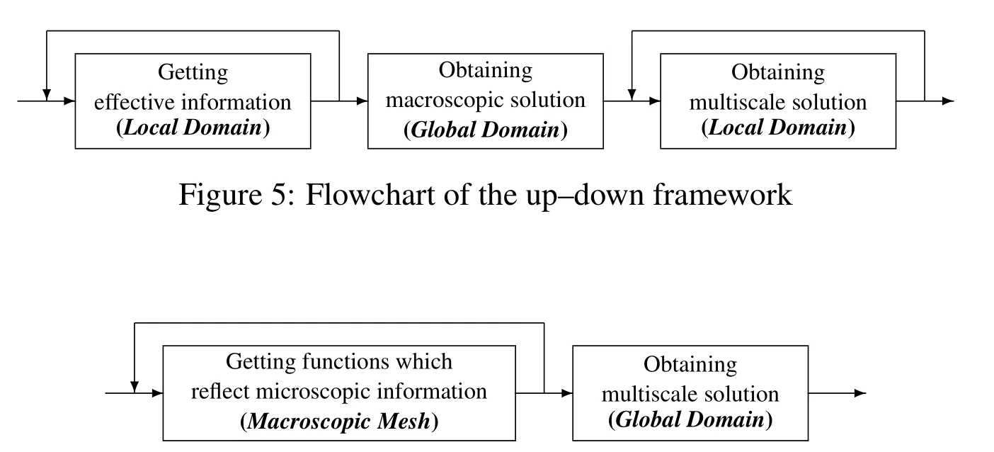
Figure 6:Flowchart of the uncoupling framework

Compared to the up–down framework,the uncoupling framework obtains the multiscale solution directly in the global domain,see Fig.6.Since the full fine scale solution of the multiscale problem cannot be solved directly in the global domain,the uncoupling framework first partitions the global domain into some small subdomains(macroscopic mesh),and tries to resolve some details of the multiscale solution in every macroscopic element independently.Special substructural functions reflecting some microscopic information are constructed in every macroscopic element and computed by solving some problems in these elements.These substructural problems can be solved in parallel because the substructural functions are independent.With the help of the substructural functions,the multiscale solution is then resolved with macroscopic mesh by solving a small discrete system.In the uncoupling framework,two levels of meshes are used,and the scale of the substructural problems depends on the macroscopic mesh size.Since the substructural functions are connected with macroscopic nodes,the multiscale solution in every fine element is derived by the macroscopic nodal solutions and the substructural functions.

Generally speaking,the two frameworks solve the multiscale problem in different ways,and provide different amount of multiscale solution.The up–down framework solves the multiscale problem in two steps.The macroscopic solution is computed first and the second step is obtaining the multiscale solution in some local domains.The multiscale solution in the global domain can also be computed when necessary.If only the macroscopic solution is required,the second step is omitted.In contrast,the uncoupling framework computes the multiscale solution directly in the global domain.In addition,the computational cost of these two frameworks is different.We compare the total degrees of freedom(DOFs)of discrete systems in these two frameworks with that of fine FEM for convenience.This is reasonable when the cost of numerical method for solving linear systems in the multiscale methods is proportional to the DOFs of the linear systems[Ming and Yue(2006)].The DOFs of the up–down framework depend on the user requirement for the multiscale solution.The DOFs are fewer than that of fine FEM when only the macroscopic solution and the multiscale solution in some small local domains are required.The DOFs will be comparable to that of fine FEM when the multiscale solution in the global domain is required.In contrast,the DOFs of the uncoupling framework are comparable to that of fine FEM because the multiscale solution in the global domain is obtained directly.Furthermore,in the up–down framework,the separation of scales is assumed,because the size of local domains for obtaining effective information should be much smaller than the macroscopic mesh size for the purpose of computing effective information more efficiently.However,the scale separation assumption is not necessary in the uncoupling framework.

Though the cost of multiscale methods in the two frameworks are comparable to that of fine FEM when the detailed multiscale solution is required,multiscale methods are still more effective than fine FEM.This is because the multiscale methods partition the multiscale problem into some independent small problems,so both the amount of computer memory and CPU time will be dramatically reduced,and it is very suitable to implement parallel computing.In contrast, fine FEM is always powerless for solving multiscale problems because of the limit of computer memory and CPU time.However we should note that the price by using multiscale methods is the accuracy of the multiscale solution.

3.2　Comparison of AHM and HMM in resolving multiscale solution

One main difference of AHM and HMM in the up–down framework is the manner they resolve multiscale solution in the local domains,as displayed in Fig.7 and Fig.8.AHM solves some auxiliary problems in a local RVE to produce auxiliary functions(e.g.χin Eq.8)which reflect microscopic information.The multiscale solution is then computed by the combination of the macroscopic solution and the microscopic auxiliary functions based on the asymptotic expansion of the multiscale solution.The number of the auxiliary problems depends on the spatial dimension.In contrast,to resolve multiscale solution,HMM solves only one problem in a local domain which takes the macroscopic solution on the boundary of the local domain as Dirichlet boundary condition.The source termfof the multiscale problem is considered in this local problem because the macroscopic solution acts as a boundary condition,while in AHM the effect of source term is represented in the macroscopic solution in the local RVE and the auxiliary problems do not consider it.For resolving multiscale solution in a local domain,HMM is more economic than AHM because only one problem should be solved.However,according to the asymptotic expansion form,AHM can provide higher–order multiscale solution when more work has been done.

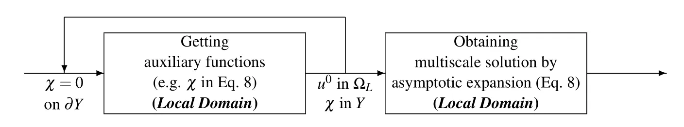
Figure 7:Flowchart of AHM in resolving multiscale solution

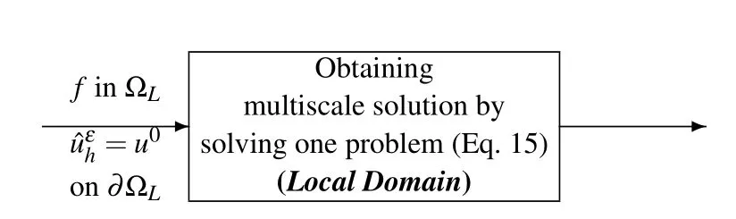
Figure 8:Flowchart of HMM in resolving multiscale solution

Though the manner to resolve multiscale solution in AHM and HMM is different,these two methods provide similar multiscale solutions in numerical computation.For simplicity,we illustrate the similarity for one–dimensional problem first.

As mentioned in section 2,to get an approximate solution of homogenized problem,HMM computes effective stiffness matrix while AHM computes effective coefficients.In fact the same strategy to obtain effective coefficients as in AHM was also adopted in HMM,see[E,Engquist,Li,Ren,and Vanden-Eijnden(2007);Yue and E(2007)].For the convenience of displaying the similarity of multiscale solutions in AHM and HMM,it is assumed that the same macroscopic solution has been obtained by these two methods.

Letu0be the numerical solution of the homogenized problem.To resolve multiscale solution,HMM needs to solve

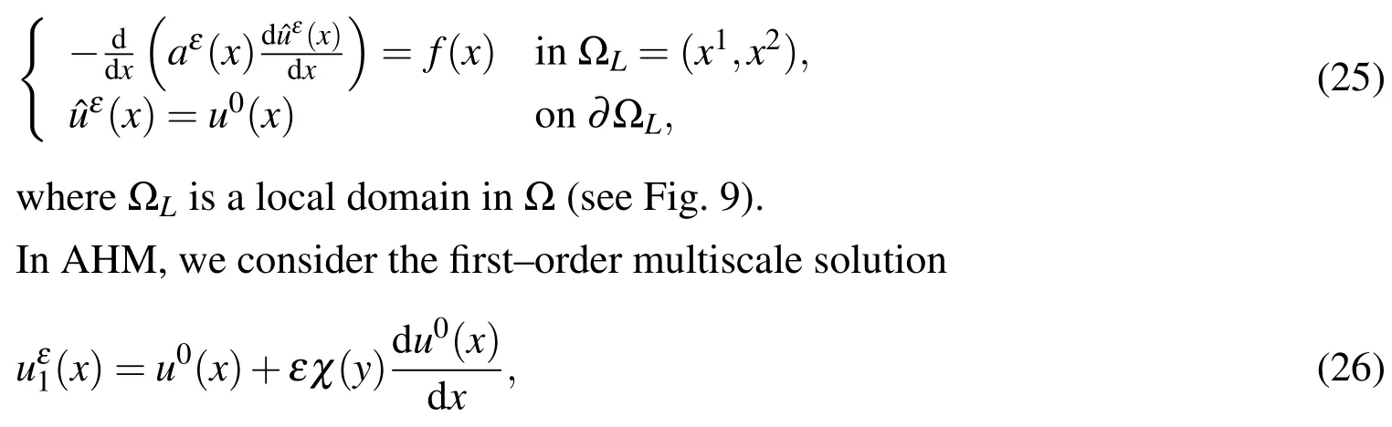
whereχis the first–order auxiliary function and is the solution of the following problem

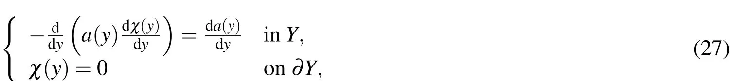
whereY=(0,1)is the unit cell.

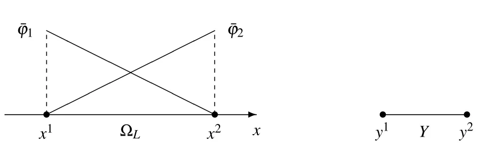
Figure 9:A diagram of ΩLandY in R

To correlate the multiscale solutions of AHM and HMM,it is assumed that ΩLis theε–cell with sizeεandYis the corresponding normalized cell of ΩL,cf.[Han,Cui,and Yu(2010)].We rewrittenχ(y)in thexcoordinates asχε(x)wherex=εy+x1.Obviouslyχεis the solution of the following problem

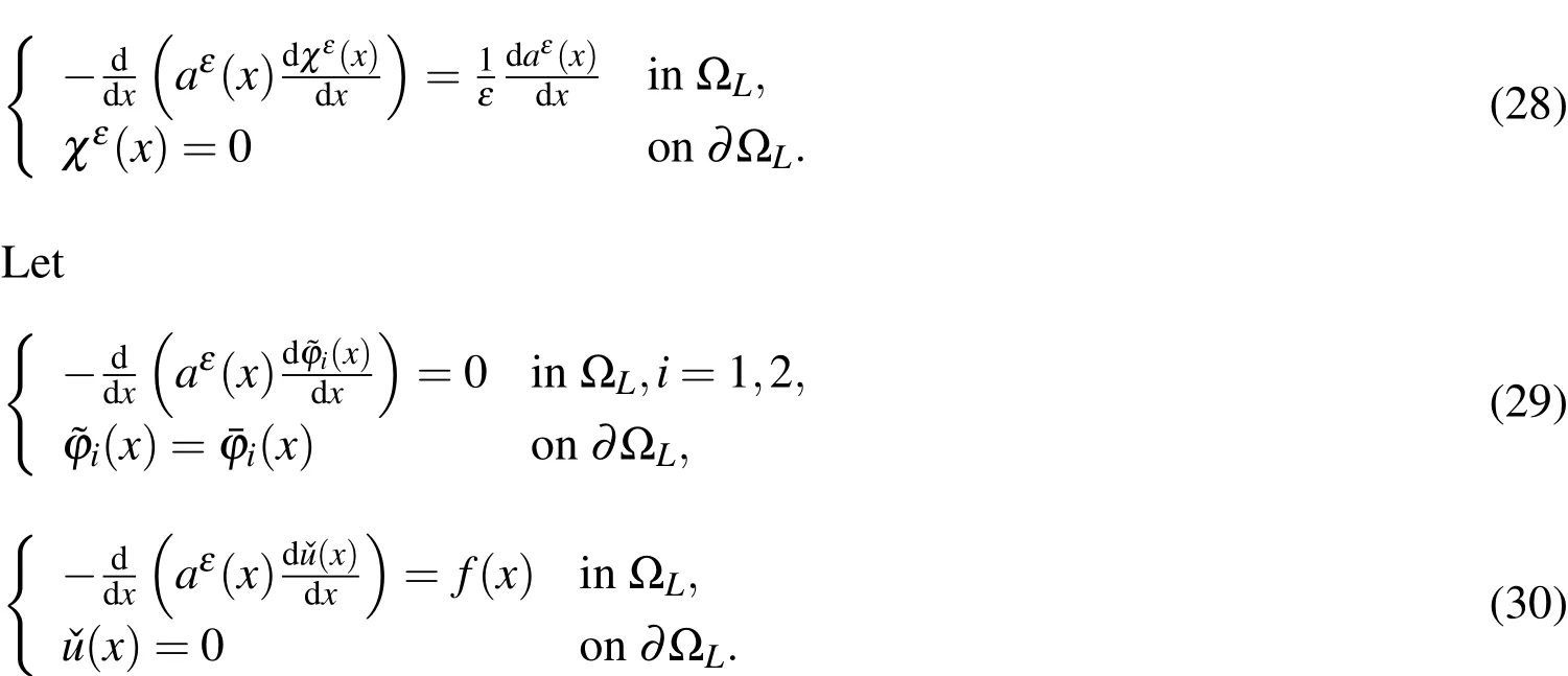
Based on the superposition principle,the multiscale solutionin HMM sat is fies

whereandare the values ofu0(x)on the left and right points of ΩL.Note thatare the multiscale base functions as same as in MsFEM,whileandare the macroscopic linear base functions(Fig.9).

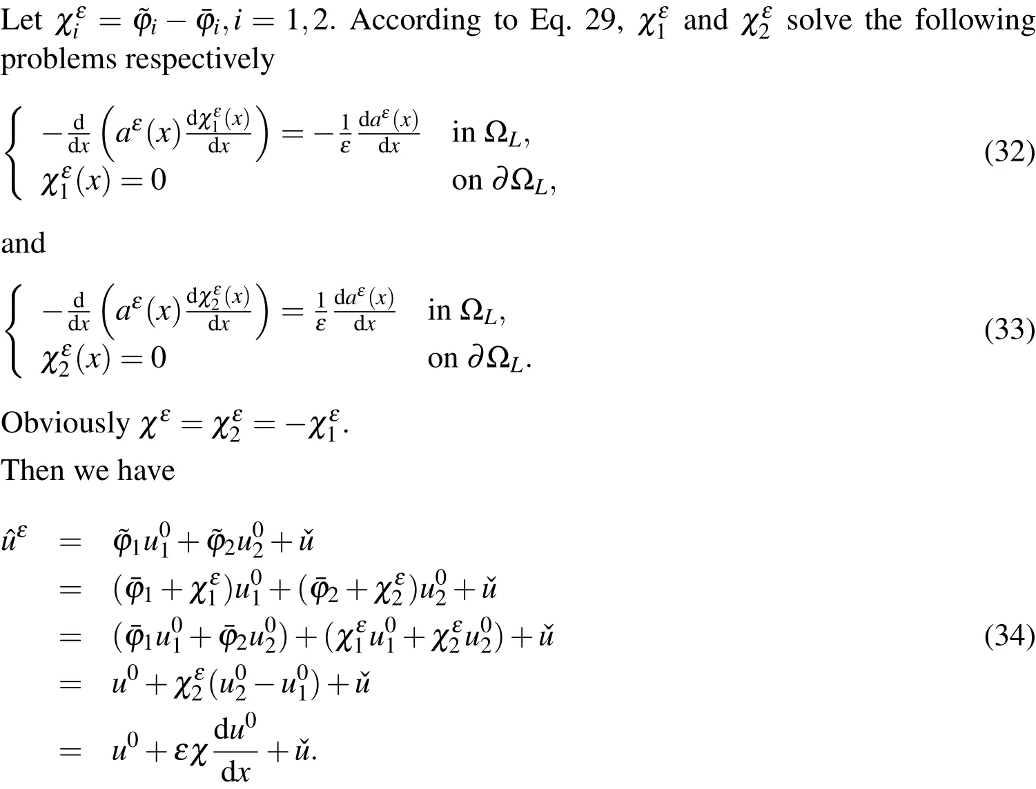
In general,the macroscopic mesh size is larger than the size of local domain ΩL.Therefore it is assumed that in AHM the macroscopic solutionu0in ΩLis approximated by linear interpolation,and its derivative is approximated by the linear combination of the derivative of linear interpolation functions with coefficientsAs in Eq.34,the multiscale solutions in HMM and AHM are equivalent in computation when ignoring the additional partObviously it holds when there is no source term in Eq.25.It has been shown that for multiscale problems which do not contain microscopic components in the source term,it is not necessary to consider the source term in the microscopic problems[Hou and Efendiev(2009);Arbogast and Boyd(2006)].We assume that the source term is a macroscopic function.In this case HMM and AHM provide equivalent multiscale solutions.

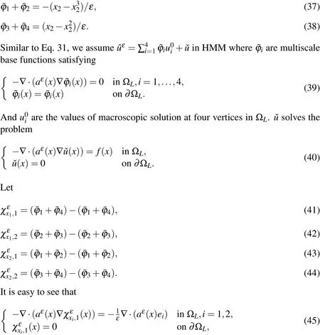
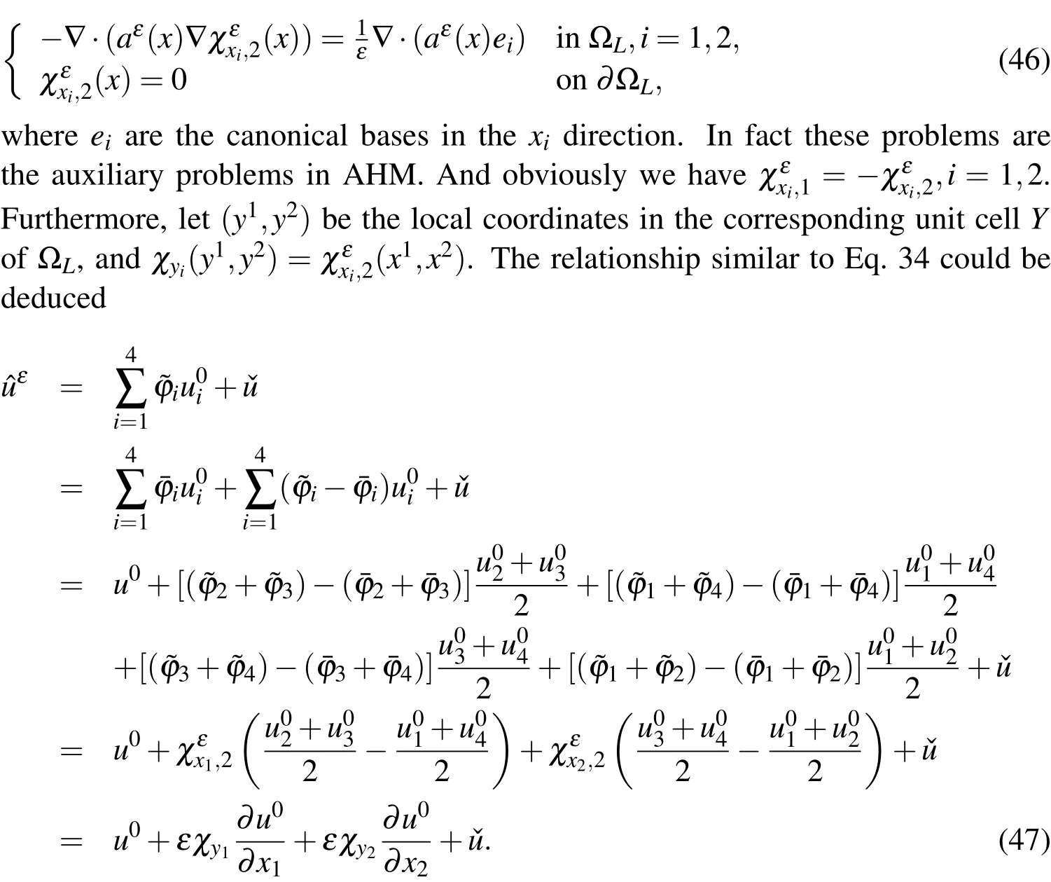
Similar result can be extended to higher–dimensional space and we illustrate it in

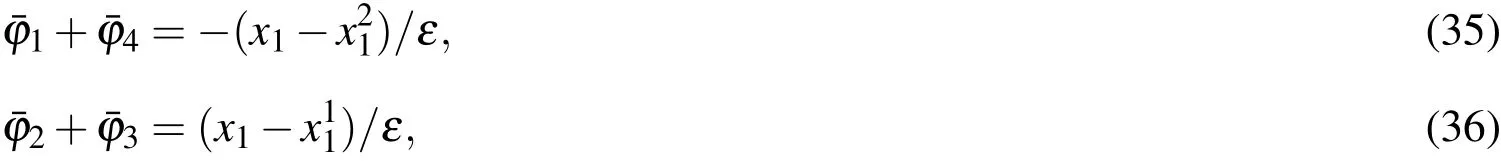
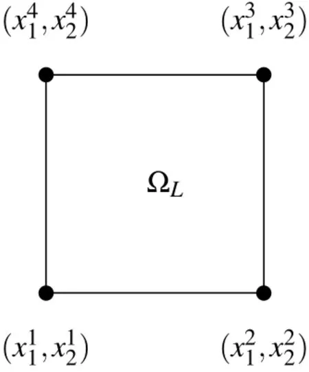
Figure 10:A diagram of ΩLin

3.3　Computational cost of different methods

Compared with fine FEM,the multiscale methods in the uncoupling framework do comparable work and resolve all the details of the multiscale solution.In contrast,we have the choice whether the multiscale solution is resolved or not by the multiscale methods in the up–down framework.The computational cost is comparable to that of fine FEM when it is necessary to obtain the multiscale solution in the global domain.However the cost will be much less when we merely concern the macroscopic solution.We compare the cost of the four multiscale methods in these two frameworks in this subsection.

As in subsection 3.1,the DOFs of the multiscale methods are compared for convenience.Tab.1 lists DOFs of the four multiscale methods for a multiscale problem with scale separation assumption.LetHandhbe the mesh sizes at the macroscaleand microscale respectively.It is assumed thatwhereδis the RVE size in AHM and HMM.In addition,the same number of nodes and the same number of quadrature points in every macroscopic element are assumed.

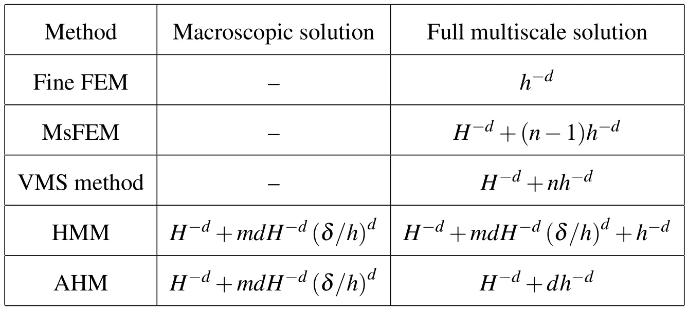
Table 1:The cost of different methods

Since the multiscale base functions in each elementin MsFEM satisfy the formula,we can solven-1 substructural problems(Eq.24)and compute the last multiscale base function by the formula.However this is not the case for VMS method.For the convenience of comparing AHM and HMM,the same RVE sizeδis assumed in AHM and HMM,and the strategy to obtain effective coefficients by solving auxiliary problems in local domains around each quadrature point is adopted in AHM.As presented in Tab.1,the cost of AHM is comparable to that of HMM for solving macroscopic solution.However,different manner to resolve multiscale solutions in HMM and AHM leads to different computational cost,and HMM is more economic than AHM.Considering the auxiliary functions could be stored and reused to construct multiscale solution,the cost to solve effective coefficients is included in the cost to resolve multiscale solution in AHM.However this is not the case for HMM.

4　Numerical experiment

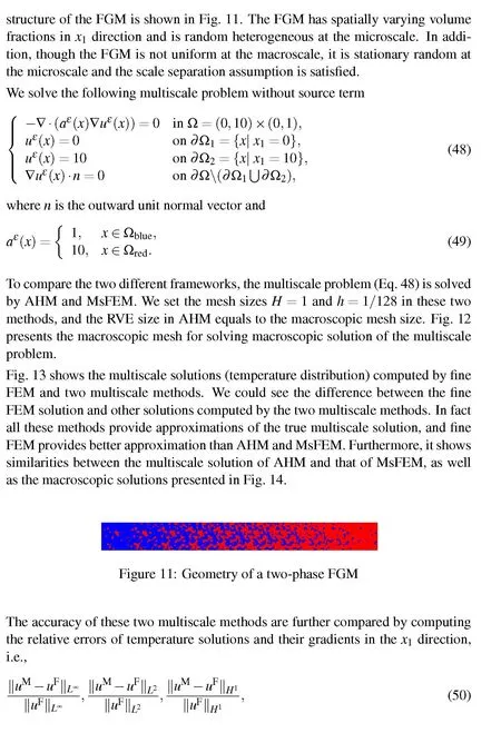
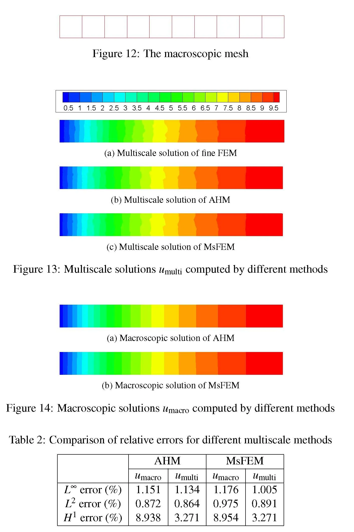
To compare the up–down framework and the uncoupling framework further,we consider a numerical example,viz.,the thermal conductivity of a two–phase functionally graded material(FGM),which is generated by random morphology description functions with computer introduced in[Vel and Goupee(2010)].The direction of fine FEM and two multiscale methods are presented in Fig.15,and macroscopic gradient solutions of these multiscale methods are shown in Fig.16.Obviously the multiscale gradient solutions given by the multiscale methods are very similar to that of fine FEM,while the macroscopic gradient solutions of the multiscale methods are not.Therefore multiscale solutions are more important in computing accurate gradient solutions.Since the computing resources are limited,only a simple numerical example is considered.However for general multiscale problems,multiscale solutions approximate solutions of the multiscale problems much better than macroscopic solutions because the latter do not contain microscopic information.

5　Conclusions

Differences and similarities of four multiscale methods for elliptic multiscale problems are shown.These methods are divided into two categories.The up–down framework includes AHM and HMM.Methods in this framework consider the macroscopic behavior of the multiscale problem with much less cost than that of fine FEM.Their cost will be comparable to that of fine FEM when all the details of the multiscale solution should be resolved.In contrast,methods in the uncoupling framework resolve the multiscale solution directly and are full fine scale solvers as fine FEM actually.VMS method and MsFEM belong to this framework.In addition,it is found that though the cost to resolve multiscale solution in AHM and HMM is different,these two methods provide similar multiscale solutions in numerical computation.Considering the feature of different multiscale methods,an effective multiscale method should be used to solve the multiscale problem according to the user requirement on the multiscale solution.

Acknowledgement:The support of the National Natural Science Foundation of China(No.90916027,No.11071196)is gratefully acknowledged.

Abdulle,A.;Schwab,C.(2005):Heterogeneous multiscale fem for diffusion problems on rough surfaces.Multiscale Modeling&Simulation,vol.3,no.1,pp.195–220.

Arabnejad,S.;Pasini,D.(2013):Mechanical properties of lattice materials via asymptotic homogenization and comparison with alternative homogenization methods.International Journal of Mechanical Sciences,vol.77,pp.249–262.

Arbogast,T.;Boyd,K.J.(2006):Subgrid upscaling and mixed multiscale finite elements.Siam Journal on Numerical Analysis,vol.44,no.3,pp.1150–1171.

Asokan,B.V.;Zabaras,N.(2006):A stochastic variational multiscale method for diffusion in heterogeneous random media.Journal of Computational Physics,vol.218,no.2,pp.654–676.

Bensoussan,A.;Lions,J.L.;Papanicolaou,G.C.(1978):Asymptotic analysis for periodic structure.Studies in Mathematics and Its Applications,vol.5.

Braess,D.(2001):Finite elements:Theory,fast solvers,and applications in solid mechanics.Cambridge University Press.

Chatzigeorgiou,G.;Efendiev,Y.;Charalambakis,N.;Lagoudas,D.C.(2012):Effective thermoelastic properties of composites with periodicity in cylindrical coordinates.International Journal of Solids and Structures,vol.49,no.18,pp.2590–2603.

Chen,F.L.;Ren,L.(2008):Application of the finite difference heterogeneous multiscale method to the richards’equation.Water Resources Research,vol.44,no.7.

Cioranescu,D.;Donato,P.(1999):An introduction to homogenization.Oxford University Press Inc.,New York.

Dong,L.T.;Atluri,S.N.(2012):Development of 3d trefftz voronoi cells with ellipsoidal voids&/or elastic/rigid inclusions for micromechanical modeling of heterogeneous materials.Cmc–Computers Materials&Continua,vol.30,no.1,pp.39–81.

Dong,L.T.;Atluri,S.N.(2012):T–trefftz voronoi cell finite elements with elastic/rigid inclusions or voids for micromechanical analysis of composite and porous materials.Cmes–Computer Modeling in Engineering&Sciences,vol.83,no.2,pp.183–219.

Dong,L.T.;Gamal,S.H.;Atluri,S.N.(2013):Stochastic macro material properties,through direct stochastic modeling of heterogeneous microstructures with randomness of constituent properties and topologies,by using trefftz computational grains(tcg).Cmc–Computers Materials&Continua,vol.37,no.1,pp.1–21.

E,W.N.;Engquist,B.(2003):The heterogeneous multiscale methods.Communications in Mathematical Sciences,vol.1,no.1,pp.87–132.

E,W.N.;Engquist,B.;Li,X.T.;Ren,W.Q.;Vanden-Eijnden,E.(2007):Heterogeneous multiscale methods:A review.Communications in Computational Physics,vol.2,no.3,pp.367–450.

E,W.N.;Ming,P.G.;Zhang,P.W.(2005):Analysis of the heterogeneous multiscale method for elliptic homogenization problems.Journal of the American Mathematical Society,vol.18,no.1,pp.121–156.

Efendiev,Y.;Chu,J.;Ginting,V.;Hou,T.Y.(2008):Flow based oversampling technique for multiscale finite element methods.Advances in Water Resources,vol.31,no.4,pp.599–608.

Efendiev,Y.;Ginting,V.;Hou,T.Y.;Ewing,R.(2006):Accurate multiscale finite element methods for two–phase flow simulations.Journal of Computational Physics,vol.220,no.1,pp.155–174.

Efendiev,Y.;Hou,T.Y.(2007):Multiscale finite element methods for porous media flows and their applications.Applied Numerical Mathematics,vol.57,no.5–7,pp.577–596.

Geers,M.G.D.;Kouznetsova,V.G.;Brekelmans,W.A.M.(2010):Multi–scale computational homogenization:Trends and challenges.Journal of Computational and Applied Mathematics,vol.234,no.7,pp.2175–2182.

Gravemeier,V.(2006):The variational multiscale method for laminar and turbulent flow.Archives of Computational Methods in Engineering,vol.13,no.2,pp.249–324.

Han,F.;Cui,J.Z.;Yu,Y.(2010):The statistical second–order two–scale method for mechanical properties of statistically inhomogeneous materials.International Journal for Numerical Methods in Engineering,vol.84,no.8,pp.972–988.

He,X.G.;Ren,L.(2006):A modified multiscale finite element method for well–driven flow problems in heterogeneous porous media.Journal of Hydrology,vol.329,no.3–4,pp.674–684.

He,X.G.;Ren,L.(2009):An adaptive multiscale finite element method for unsaturated flow problems in heterogeneous porous media.Journal of Hydrology,vol.374,no.1–2,pp.56–70.

Henning,P.;Ohlberger,M.(2010):The heterogeneous multiscale finite element method for advection–diffusion problems with rapidly oscillating coefficients and large expected drift.Networks and Heterogeneous Media,vol.5,no.4,pp.711–744.

Hou,T.Y.;Efendiev,Y.(2009):Multiscale finite element method:Theory and applications,volume 4 ofSurveys and tutorials in the applied mathematical science.Springer.

Hou,T.Y.;Wu,X.H.(1997):A multiscale finite element method for elliptic problems in composite materials and porous media.Journal of Computational Physics,vol.134,no.1,pp.169–189.

Hou,T.Y.;Wu,X.H.;Cai,Z.(1999):Convegence of a multiscale finite element method for elliptic problems with rapidly oscillating coefficients.Mathematics of Computation,vol.68,pp.913–943.

Hou,T.Y.;Wu,X.H.;Zhang,Y.(2004):Removing the cell resonance error in the multiscale finite element method via a petrov–galerkin formulation.Communications in Mathematical Sciences,vol.2,no.2,pp.185–205.

Hughes,T.J.R.(1995):Multiscale phenomena:Green’s functions,the dirichlet–to–neumann formulation,subgrid scale modles,bubbles and the origins of stabilized methods.Computer Methods in Applied Mechanics and Engineering,vol.127,pp.387–401.

Hughes,T.J.R.;Feijoo,G.R.;Mazzei,L.;Quincy,J.B.(1998):The variational multiscale method–a paradigm for computational mechanics.Computer Methods in Applied Mechanics and Engineering,vol.166,pp.3–24.

Hughes,T.J.R.;Mazzei,L.;Oberai,A.A.;Wray,A.A.(2001):The multiscale formulation of large eddy simulation:Decay of homogeneous isotropic turbulence.Physics of Fluids,vol.13,no.2,pp.505–512.

Hughes,T.J.R.;Oberai,A.A.;Mazzei,L.(2001):Large eddy simulation of turbulent channel flows by the variational multiscale method.Physics of Fluids,vol.13,no.6,pp.1784–1799.

Hughes,T.J.R.;Sangalli,G.(2007):Variational multiscale analysis:The fine–scale green’s function,projection,optimization,localization,and stabilized methods.Siam Journal on Numerical Analysis,vol.45,no.2,pp.539–557.

Kanit,T.;Forest,S.;Galliet,I.;Mounoury,V.;Jeulin,D.(2003):Determination of the size of the representative volume element for random composites:Statistical and numerical approach.International Journal of Solids and Structures,vol.40,no.13–14,pp.3647–3679.

Ma,J.A.;Temizer,I.;Wriggers,P.(2011):Random homogenization analysis in linear elasticity based on analytical bounds and estimates.International Journal of Solids and Structures,vol.48,no.2,pp.280–291.

Ma,Q.;Cui,J.Z.(2013):Second–order two–scale analysis method for the heat conductive problem with radiation boundary condition in periodical porous domain.Communications in Computational Physics,vol.14,no.4,pp.1027–1057.

Ma,X.;Zabaras,N.(2011):A stochastic mixed finite element heterogeneous multiscale method for flow in porous media.Journal of Computational Physics,vol.230,no.12,pp.4696–4722.

Ming,P.B.;Yue,X.Y.(2006):Numerical methods for multiscale elliptic problems.Journal of Computational Physics,vol.214,no.1,pp.421–445.

Oden,J.T.;Vemaganti,K.S.(2000):Estimation of local modeling error and goal–oriented adaptive modeling of heterogeneous materials i.error estimates and adaptive algorithms.Journal of Computational Physics,vol.164,no.1,pp.22–47.

Oleinik,O.A.;Shamaev,A.S.;Yosi fian,G.A.(1992):Mathematical problems in elasticity and homogenization.North–Holland,Amsterdam.

Papanicolaou,G.C.;Varadhan,S.R.S.(1981):Boundary value problems with rapidly oscillating random coefficients,volume 27,pp.835–873.North–Holland,Amsterdam,1981.

Pindera,M.J.;Khatam,H.;Drago,A.S.;Bansal,Y.(2009):Micromechanics of spatially uniform heterogeneous media:A critical review and emerging approaches.Composites Part B–Engineering,vol.40,no.5,pp.349–378.

Sab,K.;Nedjar,B.(2005):Periodization of random media and representative volume element size for linear composites.Comptes Rendus Mecanique,vol.333,no.2,pp.187–195.

Vel,S.S.;Goupee,A.J.(2010):Multiscale thermoelastic analysis of random heterogeneous materials part i:Microstructure characterization and homogenization of material properties.Computational Materials Science,vol.48,no.1,pp.22–38.

Wang,M.;Pan,N.(2008):Predictions of effective physical properties of complex multiphase materials.Materials Science&Engineering R–Reports,vol.63,no.1,pp.1–30.

Wu,Y.T.;Nie,Y.F.;Yang,Z.H.(2014):Prediction of effective properties for random heterogeneous materials with extrapolation.Archive of Applied Mechanics,vol.84,no.2,pp.247–261.

Xiao,Q.Z.;Karihaloo,B.L.(2010):Two–scale asymptotic homogenization–based finite element analysis of composite materials.Imperial College,London,2010.

Yang,S.;Yu,S.;Ryu,J.;Cho,J.M.;Kyoung,W.;Han,D.S.;Cho,M.(2013):Nonlinear multiscale modeling approach to characterize elastoplastic behavior of cnt/polymer nanocomposites considering the interphase and interfacial imperfection.International Journal of Plasticity,vol.41,pp.124–146.

Yang,Z.H.;Cui,J.Z.(2013):The statistical second–order two–scale analysis for dynamic thermo–mechanical performances of the composite structure with consistent random distribution of particles.Computational Materials Science,vol.69,pp.359–373.

Yang,Z.Q.;Cui,J.Z.;Nie,Y.F.;Ma,Q.(2012):The second–order two–scale method for heat transfer performances of periodic porous materials with interior surface radiation.Cmes–Computer Modeling in Engineering&Sciences,vol.88,no.5,pp.419–442.

Ye,S.J.;Xue,Y.Q.;Xie,C.H.(2004):Application of the multiscale finite element method to flow in heterogeneous porous media.Water Resources Research,vol.40,no.9.

Yu,Y.;Cui,J.Z.;Han,F.(2009):The statistical second–order two–scale analysis method for heat conduction performances of the composite structure with inconsistent random distribution.Computational Materials Science,vol.46,no.1,pp.151–161.

Yue,X.Y.;E,W.N.(2007):The local microscale problem in the multiscale modeling of strongly heterogeneous media:Effects of boundary conditions and cell size.Journal of Computational Physics,vol.222,no.2,pp.556–572.

Zabaras,N.;Ganapathysubramanian,B.(2009):A stochastic multiscale framework for modeling flow through random heterogeneous porous media.Journal of Computational Physics,vol.228,no.2,pp.591–618.

Zhang,H.W.;Fu,Z.D.;Wu,J.K.(2009):Coupling multiscale finite element method for consolidation analysis of heterogeneous saturated porous media.Advances in Water Resources,vol.32,no.2,pp.268–279.

Zhang,H.W.;Wu,J.K.;Fu,Z.D.(2010):Extended multiscale finite element method for elasto–plastic analysis of 2d periodic lattice truss materials.Computational Mechanics,vol.45,no.6,pp.623–635.

Zhang,H.W.;Wu,J.K.;Fu,Z.D.(2010):Extended multiscale finite element method for mechanical analysis of periodic lattice truss materials.International Journal for Multiscale Computational Engineering,vol.8,no.6,pp.597–613.

Zhikov,V.V.;Kozlov,S.M.;Oleinik,O.A.(1994):Homogenization of differential operators and integral functionals.Springer–Verlag.

Zohdi,T.I.;Wriggers,P.(2005):An introduction to computational micromechanics.Lecture notes in applied and computational mechanics.Springer–Verlag Berlin Heidelberg.