An LGDAE Method to Solve Nonlinear Cauchy Problem Without Initial Temperature
2014-04-23 05:46CheinShanLiu
Chein-Shan Liu
1 Introduction
In this paper we consider an inverse heat conduction problem(IHCP)by recovering an unknown initial condition for a nonlinear heat conduction equation under the Cauchy type boundary conditions:

whereHmay be a nonlinear function ofuandux,and the initial condition is missing to be an unknown function ofx:

For the compatibility of data we require thatf(0)=u0(0)andfx(0)=q0(0).
The sideways heat equation means the Cauchy problem for the heat conduction equation,in which the temperature and heat flux are specified as functions of time at one end of the two boundaries[Dorroh and Ru(1999);Chang,Liu and Chang(2005)].Besides the above two Cauchy boundary conditions in Eqs.(2)and(3)for a typical sideways heat equation,the present method does not need other data to recoverf(x),u(‘,t)andux(‘,t).
In the theory of partial differential equations(PDEs)there are two kinds Cauchy problems.One is for the elliptic type PDE,and another is for the parabolic type PDE;they are subjected to incomplete boundary conditions with some portion unspecifying but some portion over-specifying.Both are of the non-characteristic type initial value problems.It is well known that the Cauchy problems are highly ill-posed with a little error of input data producing a large error of numerical solution[Eld´en(1987);Eld´en,Berntsson and Reginska(2000);Qian and Fu(2007);Hao,Reinhardt and Schneider(2001);Liu(2008a,2008b);Chi,Yeih and Liu(2009);Marin(2009);Liu and Kuo(2011);Liu,Kuo and Liu(2011);Liu and Zhang(2013);Yeih,Chan,Fan,Chang and Liu(2014)].
In many industrial applications we may want to determine the temperature and heat flux on the surface of a body,but the surface itself is inaccessible for a measurement of temperature or heat flux.It may also be the case that locating a measurement device on the surface would disturb the measurements so that an incorrect temperature or heat flux is recorded.In such a situation one is restricted to internal measurements which being carried out on an accessible boundary.Berntsson(2003)has presented an example of industrial application where the sideways heat equation can be used.Sometimes we may encounter the problem that when we tackle the sideways heat equation the measurement of initial temperature is impossible,because the heat conducting device is already in service.
Wang,Cheng,Nakagawa and Yamamoto(2010)have treated the IHCP without needing of initial condition,and proved the uniqueness in determining both a boundary value and an initial value for linear sideways heat equation.Liu(2011)has studied the problem by recovering the initial condition under boundary conditions given at two boundaries.Without needing of initial condition,Liu(2014a)has proposed an iterative method to recover the heat conductivity of a nonlinear heat conduction equation,and Liu(2014b)has proposed an iterative algorithm to recover heat source under the Cauchy type boundary conditions and a final time condition.Recently,Liu and Wang(2014)have proposed a quasi-reversibility regularization method to obtain a regularized solution and convergence estimates without needing of initial temperature for the linear Cauchy problem.
As we know,there are very few methods to deal with the nonlinear sideways heat equation without initial conduction,which is very difficult to be solved numerically.In this paper we will provide a simple and yet stable numerical method to solve this highly ill-posed nonlinear Cauchy problem with multiple unknowns of initial condition and right-boundary conditions.
The outline of this paper is given as follows.In Section 2 we propose a variable transformation,such that the nonlinear Cauchy problem without initial value becomes a nonlinear inverse heat source problem with zero initial value.Sections 3-5 devote to the development of a Lie-group differential algebraic equations(LGDAE)method and a numerical algorithm based on the Lie-groupGL(N,R)for the general DAEs system.In Section 6,we view the nonlinear inverse heat source problem in Section 2 as a special type nonlinear DAEs,and derive a numerical algorithm to solve the resultant DAEs.Numerical examples are given in Section 7 to validate the efficiency and accuracy of LGDAE.Some conclusions are drawn in the final Section 8.
2 A variable transformation and the numerical method of lines
Let

wheref(x)is an unknown function of initial temperature to be determined.From Eqs.(1)-(4)it follows that

whereF(x)=f00(x)is viewed as an unknown spatially-dependent function of heat source.
Here,a novel method of Lie-group differential algebraic equations(LGDAE)method will be developed to estimate the unknown heat sourceF(x)and unknown initial conditionf(x),which merely requires the boundary conditions and initial condition given by Eqs.(7)-(9)for estimatingF(x),and the boundary conditions given by Eqs.(2)and(3)for estimatingf(x).
The numerical method of lines is simple that for a given system of PDEs we discretize all but one of the independent variables.The semi-discrete procedure yields a coupled system of ordinary differential equations(ODEs),which are then being numerically integrated to obtain solution.For Eq.(6)we adopt the numerical method of lines to discretize the time coordinatetbyti,by lettingSi(x)=Tx(x,ti)andTi(x)=T(x,ti),and keepxa continuous variable,whereti=(i− 1)∆t=(i−1)tf/(m−1)and∆tis a uniform time-stepsize.Such that we can derive

whereHi=H(x,ti,Ti+f,Si+f0)=H(x,ti,Ti+Tm+1,Si+Sm+1)byde finingTm+1(x)=f(x)andSm+1(x)=f0(x).If we can knowF(x),we can integrate Eqs.(10)-(14)by using the group preserving scheme(GPS)developed by Liu(2001),where we denote the spatial stepsize by∆x=‘/(n−1).Besides the above ODEs we have a constraint equation:

which is obtained from Eq.(9).Here,we must emphasize thatT1(x)plays two roles:satisfying Eqs.(10)and(15).Recently,Liu(2014c)has argued that the Cauchy problem of heat equation is solvable,because the field equation is extend able to the initial time by using the concept of analytic continuation.The above technique to treat the temperatureT1(x)on the line at initial time is indeed an application of the analytic continuation method.
3 Lie-group differential algebraic equations method

Eqs.(10)-(15)constitute a set of differential algebraic equations(DAEs)withF(x)to be an unknown function.Here we generalize the above DAEs to and propose a novel method to solve the above DAEs,which govern the evolution ofN+qvariablesxi,i=1,...,Nandyj,j=1,...,qwithNordinary differential equations(ODEs)andqnonlinear algebraic equations(NAEs).The vector y in Eq.(16)is viewed as unknown parameter.We have replacedxin Eqs.(10)-(15)bytfor a purpose of the demonstration for the general DAEs written in a time domain.There are many numerical methods used to solve ODEs.But only a few is used to solve DAEs.The present technique used to solve the inverse heat source problem is a DAE method,whose pre-requirement is however a powerful and stable method to solve the DAEs as to be described below.The DAEs are more difficult to be solved numerically than ODEs and NAEs.
Liu(2013a)was the first to find the essential form forn-dimensional nonlinear ordinary differential equations(ODEs)in terms of the Lie-algebragl(n,R)ofGL(n,R),and developed a very effective Lie-groupGL(n,R)preserving scheme to solve ODEs.Then,Liu(2013b)developed a Lie-groupGL(n,R)preserving scheme to solve ODEs by assuming that the coefficient matrix is constant in a small time incremental step.Moreover,Liu(2013c)has developed a powerful numerical method to solve the nonlinear DAEs based on the above Lie-groupGL(n,R)preserving scheme,which is named the Lie-group DAE(LGDAE)method.It is also interesting that the LGDAE can be used to solve the sliding control problem by Liu(2014d).Liu and Atluri(2013)have employed the LGDAE to solve the problem of numerical differential of a noisy signal.
4 The GL(N,R)structure of differential equations system
The Lie-group is a differentiable manifold,which is endowed with a group structure that is compatible with the underlying topology of the manifold.The Lie-group solver can provide a better algorithm that retains the orbit generated from numerical solution on the manifold which is associated with the Lie-group.
The general linear group is a Lie group,whose manifold is an open subsetGL(N,R):={G∈RN×N|detG 6=0}of the linear space of allN×Nnon-singular matrices.Thus,GL(N,R)is also anN×N-dimensional manifold.
The general linear groupGL(N,R)gives uniquely a real Lie-algebragl(N,R).Consider a one-parameter subgroup G(t),t∈R,of the general linear groupGL(N,R),which is a curve passing through the group identity att=0,

and which operates from the left on theN-dimensional Euclidean space RN,resulting in a Lie-group equation:

where A∈gl(N,R)is the corresponding Lie-algebra.
Here we give a new form of the dynamics in Eq.(16)from theGL(N,R)Lie-group structure.In order to fit the form in Eq.(19),the vector field f on the right-hand side of Eq.(16)can be written as

where

is the coefficient matrix.Here u⊗y denotes the dyadic operation of u and y,i.e.,(u⊗y)z=y·zu.
Because the coefficient matrix A is well-defined for kxk>0,the Lie-group element G generated from the above dynamical system(20)with˙G=AG satis fies det G(t)6=0,such that G∈GL(N,R).
5 An implicit GL(N,R)Lie-group scheme
Eq.(20)is a new starting point for the development of the Lie-groupGL(N,R)scheme.In order to develop a numerical scheme from Eqs.(20)and(21),we suppose that the coefficient matrix A is constant with

being two constant vectors,which can be obtained by taking the values of f and x at a suitable mid-point of¯t∈[t0=0,t],wheret≤t0+handhis a small time stepsize.Thus from Eqs.(20)and(21)it follows that

Let

and Eq.(23)becomes

At the same time,from the above two equations we can derive the following ODE forw:

where

is supposed to be a constant value in a small time interval oft∈[t0,t0+h].Thus,we have

wherew0=b·x0.
Inserting Eq.(28)forw(t)into Eq.(25)and integrating the resultant equation we can obtain

where x0is the initial value of x at an initial timet=t0=0,and


Then we can prove

which means that G is a Lie-group element ofGL(N,R).
Accordingly,we can develop the following scheme based on the Lie-groupGL(N,R)for solving the ODEs in Eq.(16):
(i)Give 0≤θ≤1.
(ii)Give an initial value of x0at an initial timet=t0and a time stepsizeh.
(iii)Fork=0,1,...,we repeat the following computations to a specified terminal timet=tf:

With the above xk+1generated from an Euler step as an initial guess we iteratively solve the new xk+1by
在配电网中,由于受到变电站选址和通道受限的影响,往往需要对已有变电站进行升级改造,以满足长期负荷增长需求;但由于现场施工条件限制和电网安全规程要求,不得不选择全站停电改造,且改造周期较长。以某地市公司110 kV变电站为例,停电时间长达5个月,在此改造期间,配电网运行压力巨大,能否平稳度过负荷高峰时期,缺乏理论支撑和可行性论证,施工中能否安排全站停电进行升级改造缺乏有效规程参考和指导意见。

If zk+1converges according to a given stopping criterion:

then go to(iii)to the next time step;otherwise,let xk+1=zk+1and go to Eq.(34).In the above ykis viewed as a constant vector within a small time step.In order to determine ykthe present Lie-group scheme is coupled with the following Newton iterative scheme.
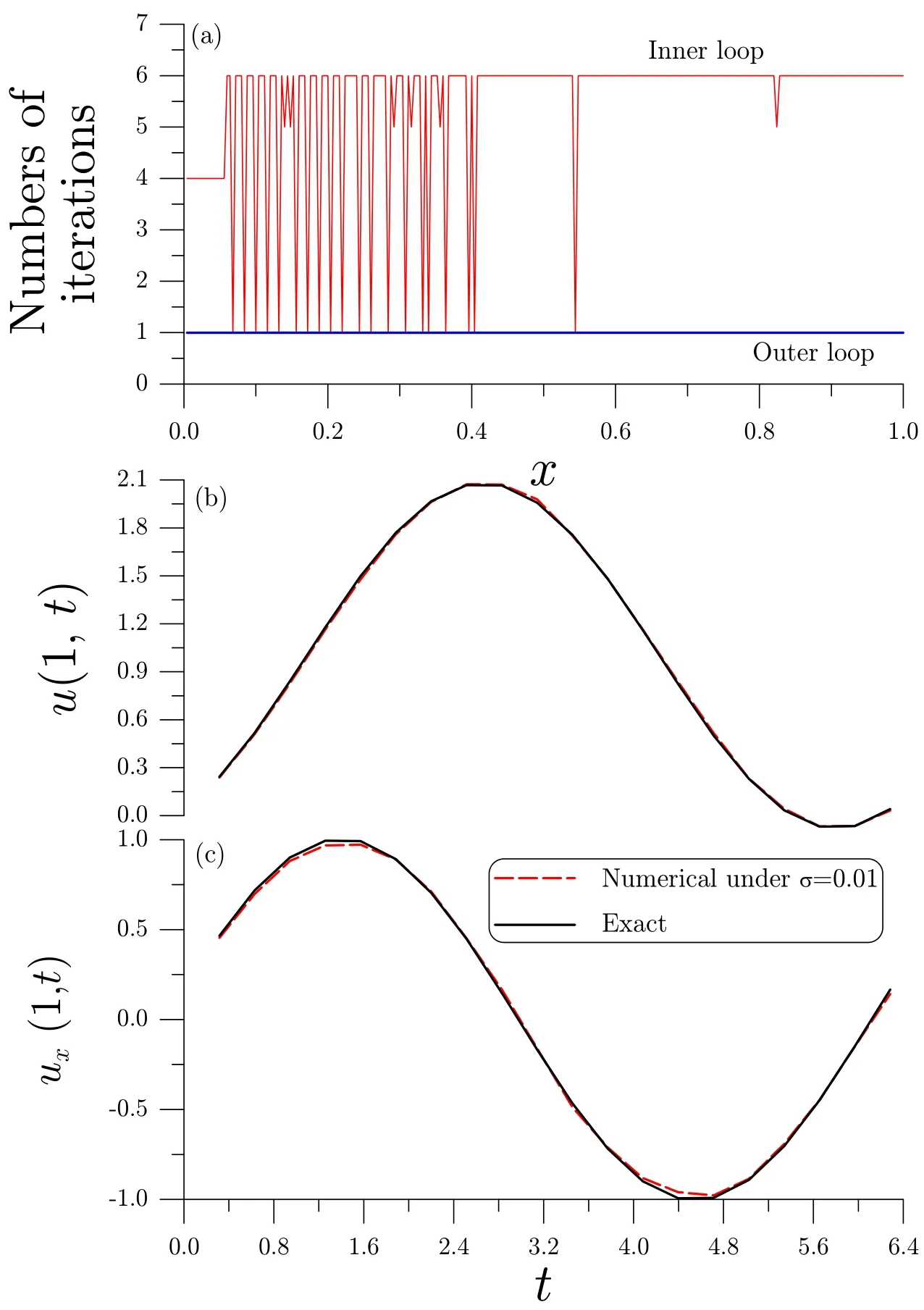
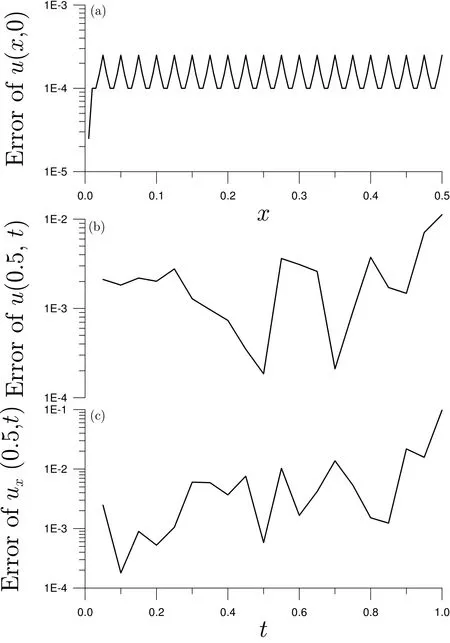
Within a small time step we can suppose that the variablesyj,j=1,...,qare constant in the interval oftk until the following convergence criterion is satisfied: otherwise,go to Eq.(34)and insert the new.In above,the componentBijof the Jacobian matrix B is given by∂Fi/∂yj. The numerical scheme is a combination of the Lie-group method based onGL(N,R)and the Newton iterative method to solve the DAEs in Eqs.(16)and(17),which is called the Lie-group differential algebraic equations(LGDAE)method. Now we apply the above LGDAE withN=2m+2 andq=1 to solve T=(T1,...,Tm,Tm+1)T,S=(S1,...,Sm,Sm+1)Tand hencef(x)=Tm+1(x)through Eqs.(10)-(14),and simultaneously solve the unknown functionF(x)through Eq.(15)by the Newton iterative method.The numerical processes are given below: (i)Give an initial guess ofF0,for example,F0=0. (ii)Give initial conditions of T0and S0at an initial pointx=0 and a spatial stepsize∆x. (iii)Fork=0,1,...,we repeat the following computations to a terminal pointx=‘: where fkdenotes thek-th step value of the right-hand side in Eqs.(11)-(14).With the above Tk+1and Sk+1generated from an Euler step as an initial guess we then iteratively solve the new Tk+1and Sk+1by then go to(iv);otherwise,let Tk+1=and Sk+1=and go to Eq.(38).(iv)Forj=0,1,...,we repeat the following computations: where the prime denotes the differential with respect toF,and Obviously,from Eqs.(11)-(14)one has=(−1m,1)T=(−1,...,−1,1)T,where 1m=(1,...,1)T.Ifconverges according to then go to(iii)for the next step;otherwise,letand go to Eq.(38).The above iteration with ε1as a convergence criterion is called the outer iteration or outer loop,while that with ε2as a convergence criterion is called the inner iteration or inner loop.In the computations given below the maximum numbers of iterations for inner and outer iterations are fixed to be 100 and 200,respectively.In all the computations given below we will fix the weighting factor θ to be θ =1/2. In this section we test the proposed LGDAE in the solution of the Cauchy problem without initial condition.All the required left boundary conditions can be derived from exact solutions.Here we consider the noise being imposed on the left-boundary conditions by whereR(i)are random numbers in[−1,1],and σ is the intensity of noise. We define the root-mean-square-error(RMSE)in the recoveries of initial condition and right boundary conditions by wheremis the number of the discretized times andnis the number of steps used in the integration of the governing equations along thex-direction.Whenu∗(xj,0),u∗(‘,tk)andu∗x(‘,tk)denote the numerical solutions,u(xj,0),u(‘,tk)andux(‘,tk)denote the exact solutions. In this example the exact solution ofuis Under the convergence criteria ε2=10−12for inner iterations and ε1=10−4for outer iterations,we apply the LGDAE to solve the above problem,where the following parameters:m=21,n=251 and a noise with σ=0.01 are considered.As shown in Fig.1(a),the numbers of iterations are few with one,four or six for inner iterations and one for outer iterations.It shows that the LGDAE is a highly efficient method,which is convergent very fast.In Fig.1(b)we compare the recovered temperature with the exact one,and in Fig.1(c)we compare the recovered heat flux with the exact one,which are almost coincident.Thus we plot the numerical error in Fig.2,of which the maximum error and RMSE1 of initial temperatures are,respectively,1.7×10−2and 4×10⁻³,the maximum error and RMSE2 of right-end temperatures are,respectively,2.1×10−2and 9.9×10⁻³,and the maximum error and RMSE3 of right-end heat fluxes are 3.4×10⁻²and 1.6×10⁻²,respectively. Figure 1:For example 1:(a)the numbers of inner and outer iterations,(b)comparing right-end temperatures,and(c)comparing right-end heat fluxes. Figure 2:For example 1 showing the numerical errors of(a)initial temperature,(b)right-end temperature,and(c)right-end heat flux. Next,we assume that the exact solution ofuis Under the following parameters:m=31,n=251 and under a noise with σ=0.01,we use the LGDAE to solve the above inverse problem to recover the initial temperature and two right-end boundary conditions as shown in Fig.3,of which the maximum error and RMSE1 of initial temperatures are,respectively,1.3×10−2and 7.9×10⁻³,the maximum error and RMSE2 of right-end temperatures are,respectively,5.6×10−3and 1.3×10⁻³,and the maximum error and RMSE3 of right-end heat fluxes are 3.4×10⁻²and 9.1×10⁻³,respectively. Then we consider a nonlinear heat conduction equation: where the exact solution is supposed to be Inserting Eq.(5)into Eq.(49)we can obtain Now we can apply the LGDAE to solve the above equation to findf(x)andF(x)under the following parameters:m=21,n=251 and under a noise with σ=0.005.The numerical errors are shown in Fig.4,of which the maximum error and RMSE1 of initial temperatures are,respectively,5.2×10−2and 2.4×10⁻²,the maximum error and RMSE2 of right-end temperatures are,respectively,6.5×10−3and 3×10⁻³,and the maximum error and RMSE3 of right-end heat fluxes are 6×10⁻²and 1.7×10⁻²,respectively. Figure 3:For example 2 showing the numerical errors of(a)initial temperature,(b)right-end temperature,and(c)right-end heat flux. Figure 4:For nonlinear example 3 showing the numerical errors of(a)initial temperature,(b)right-end temperature,and(c)right-end heat flux. Figure 5:For example 4 of Burgers equation showing the numerical errors of(a)initial temperature,(b)right-end temperature,and(c)right-end heat flux. Finally,we consider a nonlinear Burgers equation: where the exact solution is supposed to be Inserting Eq.(5)into Eq.(52)we can obtain When we apply the LGDAE to solve the above inverse problem under the following parameters:m=21,n=101 and under a noise with σ=0.002,the numerical errors are shown in Fig.5,of which the maximum error and RMSE1 of initial temperatures are,respectively,2.5×10−4and 1.6×10⁻⁴,the maximum error and RMSE2 of right-end temperatures are,respectively,1.1×10−2and 3.5×10⁻³,and the maximum error and RMSE3 of right-end heat fluxes are,respectively,9.8×10−2and 2.3×10⁻². There are very few methods that can solve the nonlinear sideways heat conduction problem without initial condition,which is a highly ill-posed inverse heat conduction problem.The existing methods in the literature are most restricted to solve linear Cauchy problems.We have transformed the nonlinear Cauchy problem without initial condition into a nonlinear heat source identification problem with a zero initial condition.Then,we have explained that the discretized version after using the numerical method of lines is a set of nonlinear differential algebraic equations,for which we have used the newly developed LGDAE to solve the unknown initial temperature and recover boundary temperature and heat flux on the right-end.Although under a large noisy disturbance on the Cauchy data,the accuracy and efficiency of numerical solutions were con firmed by comparing the recovered results with exact solutions. Acknowledgement:Taiwan’s National Science Council project NSC-102-2221-E-002-125-MY3 and the 2011 Outstanding Research Award,granted to the author,are highly appreciated. Berntsson,F.(2003):Sequential solution of the sideways heat equation by windowing of the data.Inv.Prob.Sci.Eng.,vol.11,pp.91-103. Chang,C.W.;Liu,C.-S.;Chang,J.R.(2005):A group preserving scheme for inverse heat conduction problems.CMES:Computer Modeling in Engineering&Sciences,vol.10,pp.13-38. Chi,C.C.;Yeih,W.;Liu,C.-S.(2009):A novel method for solving the Cauchy problem of Laplace equation using the fictitious time integration method.CMES:Computer Modeling in Engineering&Sciences,vol.47,pp.167-190. Dorroh,J.R.;Ru,X.(1999):The application of the method of quasi-reversibility to the sideways heat equation.J.Math.Anal.Appl.,vol.236,pp.503-519. Eld´en,L.(1987):Approximations for a Cauchy problem for the heat equation.Inverse Problem,vol.3,pp.263-273. Eld´en,L.;Berntsson,F.;Reginska,T.(2000):Wavelet and Fourier methods for solving the sideways heat equation.SIAM J.Sci.Comput.,vol.21,pp.2187-2205. Hao,D.N.;Reinhardt,H.J.;Schneider,A.(2001):Numerical solution to a sideways parabolic equation.Int.J.Numer.Meth.Engng.,vol.50,pp.1253-1267. Liu,C.-S.(2001):Cone of non-linear dynamical system and group preserving schemes,Int.J.Non-Linear Mech.,vol.36,pp.1047-1068. Liu,C.-S.(2008a):A highly accurate MCTM for inverse Cauchy problems of Laplace equation in arbitrary plane domains.CMES:Computer Modeling in Engineering&Sciences,vol.35,pp.91-111. Liu,C.-S.(2008b):A highly accurate MCTM for direct and inverse problems of biharmonic equation in arbitrary plane domains.CMES:Computer Modeling in Engineering&Sciences,vol.30,pp.65-75. Liu,C.-S.(2011):A self-adaptive LGSM to recover initial condition or heat source of one-dimensional heat conduction equation by using only minimal boundary thermal data.Int.J.Heat Mass Transfer,vol.54,pp.1305-1312. Liu,C.-S.(2013a):A method of Lie-symmetryGL(n,R)for solving non-linear dynamical systems.Int.J.Non-Linear Mech.,vol.52,pp.85-95. Liu,C.-S.(2013b):A state feedback controller used to solve an ill-posed linear system by aGL(n,R)iterative algorithm.Commu.Numer.Anal.,vol.2013,Article ID cna-00181,22 pages. Liu,C.-S.(2013c):Solving nonlinear differential algebraic equations by an implicitGL(n,R)Lie-group method.J.Appl.Math.,vol.2013,ID 987905,8 pages. Liu,C.-S.(2014a):An iterative method to recover heat conductivity function of a nonlinear heat conduction equation.Num.Heat Transfer,B:Fundamentals,vol.65,pp.80-101. Liu,C.-S.(2014b):An iterative algorithm for identifying heat source by using a DQ and a Lie-group method.Inv.Prob.Sci.Eng.,dx.doi.org/10.1080/17415977.2014.880907. Liu,C.-S.(2014c):Lie-group differential algebraic equations method to recover heat source in a Cauchy problem with analytic continuation data.Int.J.Heat Mass Transfer,vol.78,pp.538-547. Liu,C.-S.(2014d):A new sliding control strategy for nonlinear system solved by the Lie-group differential algebraic equation method.Commun.Nonlinear Sci.Numer.Simulat.,vol.19,pp.2012-2038. Liu,C.-S.;Atluri,S.N.(2013):AGL(n,R)differential algebraic equation method for numerical differentiation of noisy signal.CMES:Computer Modeling in Engineering&Sciences,vol.92,pp.213-239. Liu,C.-S.;Kuo,C.L.(2011):A spring-damping regularization and a novel Liegroup integration method for nonlinear inverse Cauchy problems.CMES:Computer Modeling in Engineering&Sciences,vol.77,pp.57-80. Liu,C.-S.;Kuo,C.L.;Liu D.(2011):The spring-damping regularization method and the Lie-group shooting method for inverse Cauchy problems.CMC:Computers,Materials&Continua,vol.24,pp.105-123. Liu,J.C.;Wang,J.G.(2014):Cauchy problem for the heat equation in a bounded domain without initial value.CMES:Computer Modeling in Engineering&Sciences,vol.97,pp.437-462. Liu,J.C.;Zhang,Q.G.(2013):Cauchy problem for the Laplace equation in 2D and 3D doubly connected domains.CMES:Computer Modeling in Engineering&Sciences,vol.93,pp.203-220. Marin,L.(2009):An alternating iterative MFS algorithm for the Cauchy problem in two-dimensional anisotropic heat conduction.CMC:Computers,Materials&Continua,vol.12,pp.71-99. Qian,Z.;Fu,C.L.(2007):Semi-discrete central difference method for determining surface heat flux of IHCP.J.Korean Math.Soc.,vol.44,pp.1397-1415. Wang,Y.;Cheng,J.;Nakagawa,J.;Yamamoto,M.(2010):A numerical method for solving the inverse heat conduction problem without initial value.Inv.Prob.Sci.Eng.,vol.18,pp.655-671. Yeih,W.;Liu,C.-S.;Kuo,C.L.,Atluri,S.N.(2010):On solving the direct/inverse Cauchy problems of Laplace equation in a multiply connected domain,using the generalized multiple-source-point boundary-collocation Trefftz method&characteristic lengths.CMC:Computers,Materials&Continua,vol.17,pp.275-302. Yeih,W.;Chan,I.Y.;Fan,C.M.;Chang,J.J.;Liu,C.-S.(2014):Solving the Cauchy problem of the nonlinear steady-state heat equation using double iteration process.CMES:Computer Modeling in Engineering&Sciences,vol.99,pp.169-194.
6 Numerical algorithm


7 Numerical tests


7.1 Example 1


7.2 Example 2

7.3 Example 3


7.4 Example 4


8 Conclusions
猜你喜欢
现代仪器与医疗(2022年3期)2022-08-12
世界汽车(2022年3期)2022-05-23
电子乐园·下旬刊(2022年6期)2022-05-16
青海农技推广(2022年4期)2022-02-15
销售与市场(营销版)(2021年4期)2021-04-16
四川劳动保障(2021年3期)2021-01-27
世界汽车(2020年6期)2020-12-28
中国工程咨询(2015年5期)2015-02-16
云南电力技术(2015年1期)2015-02-10
中国卫生(2014年11期)2014-11-12