
Influence of Design Margin on Operation Optimization and Control Performance of Chemical Processes*
2014-07-18 11:56XUFeng许锋JIANGHuirong蒋慧蓉WANGRui王锐andLUOXionglin罗雄麟
XU Feng (许锋), JIANG Huirong (蒋慧蓉), WANG Rui (王锐) and LUO Xionglin (罗雄麟)**
Research Institute of Automation, China University of Petroleum, Beijing 102249, China
Influence of Design Margin on Operation Optimization and Control Performance of Chemical Processes*
XU Feng (许锋), JIANG Huirong (蒋慧蓉), WANG Rui (王锐) and LUO Xionglin (罗雄麟)**
Research Institute of Automation, China University of Petroleum, Beijing 102249, China
Operation optimization is an effective method to explore potential economic benefits for existing plants. The maximum potential benefit from operation optimization is determined by the distances between current operating point and process constraints, which is related to the margins of design variables. Because of various disturbances in chemical processes, some distances must be reserved for fluctuations of process variables and the optimum operating point is not on some process constraints. Thus the benefit of steady-state optimization can not be fully achieved while that of dynamic optimization can be really achieved. In this study, the steady-state optimization and dynamic optimization are used, and the potential benefit is divided into achievable benefit for profit and unachievable benefit for control. The fluid catalytic cracking unit (FCCU) is used for case study. With the analysis on how the margins of design variables influence the economic benefit and control performance, the bottlenecks of process design are found and appropriate control structure can be selected.
design margin, operation optimization, control performance, bottleneck, fluid catalytic cracking unit (FCCU)
1 INTRODUCTION
Operation optimization is an effective method to explore potential economic benefits for existing chemical plants, while the economic benefits from operation optimization depend on the margins of design variables. According to the demand for optimal design of chemical process, the steady-state operating point of the optimal design generally lies on the boundaries of process constraints. In operations, process variables should be restricted within active constraints on condition that they are “hard”. However, the effect of disturbances and uncertainties in real processes usually perturb the plant from the desired steady-state optimum operating point, violating some active constrains, so the plant can not run at the desired steady-state optimum operating point. To ensure operating feasibility and production goals, sufficient margins must be added on the design variables, then the operating point will move into the feasible region and there are proper distances between current operating point and active constraints. The magnitudes of the distances lead to the back-off of process economic performance but provide free space for operation optimization.
The margins of design variables will directly influence process operation and control performance. When process conditions change or disturbances occur, the process variables change with time dynamically, which are generally damped oscillation processes because of the process control system. The dynamic process must be considered in design margins, otherwise the process control system can not work. Xu and Luo [1-4] have pointed out that, for conventional proportional-integral-differential (PID) control or for model predictive control, design margins for control and operation must be considered and their sizes are related to process control system. The better control performance is requested, the more margins are required. Larger margin may bring more flexibility in operation and control, but requires larger equipment investment and operating costs.
A number of methodologies have been developed for addressing the interactions between process design and process control. Previous researches about margin analysis, operatability and control performance evaluation, and integration of process design and control are as follows.
(1) Process controllability assessment. When considering process uncertainty, the evaluation of open and closed-loop controllability indicators of different process designs allows the comparison and classification of alternatives in terms of operational characteristics, such as the metric of open-loop controllability [5], dynamic economic impact of disturbance and uncertain parameters [6, 7], and flexibility and resilience analysis [8-10].
(2) Simultaneous design and control. More systematic efforts are on the context of interactions of design and control to design economically optimal processes that could operate in an efficient dynamic mode within an envelope around the nominal point. Economicsbased performance index and control performance are usually considered based on dynamic model, and possible disturbances and uncertainties are taken into account. Dynamic optimization is employed in order to determine the most economic process design and control system that satisfies all dynamic operability constraints. There are several aspects about the problem such ascontrol algorithm, optimization algorithm, quantification of disturbances and parametric uncertainty. After years of development, control algorithms have extended from conventional PID control [11] to optimal control [12, 13], predictive control [14], and internal model control [15]. Optimization algorithms have developed from the conventional nonlinear programming [16] to the heuristic particle swarm optimization (PSO) algorithm [17], and the robust control tools based on Lyapunov theory and structured singular value analysis are used to estimate the bounds on process worst-case variability, process feasibility, and process stability [18-20]. The applied processes have extended from distillation column [21] to polymerization reactor [22-24]), crystallization reactor [25] and so on.
(3) Margin analysis and control design based on dynamic models. Xu and Luo [1-4] have integrated margin analysis methods into the optimized process and control design. It is found that the design margin should be divided into steady-state margin and dynamic margin, and the dynamic margin is necessary for control and is related to control system. In process design the control performance and design margins should be considered as a whole in order to fulfill process demand and achieve good control performance.
In the presence of design margins, the distances between current operating point and active constraints provide certain space for operation optimization. The steady-state operation optimization is often used for more economic benefit. However, there are various disturbances and process variables always vary in chemical processes, and some distances between the optimum operating point and process constraints must be reserved for dynamic regulations of control system, so the operation optimization can not fully explore the space from design margins and the benefit of the steady-state operation optimization can not be fully achieved. Only the benefit from dynamic operation optimization considering dynamic responses of process variables can be really achieved.
In this paper, steady-state optimization and dynamic optimization are used to evaluate the potential benefit of FCCU, which is divided into achievable benefit for profit and unachievable benefit for control. To explore how the margins of design variable influence the economic benefit and control performance, the bottlenecks of process design could be found and appropriate control structure could be selected.
2 OPERATION OPTIMIZATION AND DESIGN MARGIN
An ideal process should be designed to achieve optimal economic performance while meeting all process constraints. The optimal design is given by

where vector χ represents the state variables, d represents the design variables, u represents the manipulation variables, f(·) the equations of process model, g(·) the equations of process constraints, and F is the objective function of optimal design, involving equipment investment cost and operating cost. With the steady-be obtained.
To solve the optimal design problem, we define the Lagrange function as
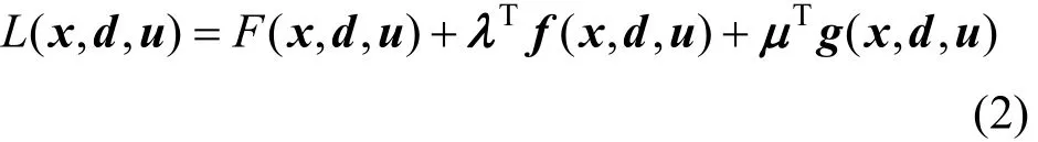
where λ is the Lagrange multiplier vector of equality constraints and μ is the Lagrange multiplier vector of inequality constraints.
Let i and j represent the active set and non-active set of inequality constraints respectively. For the active set, the optimal solution is on the boundaries of process constraints gi(·)=0, with corresponding Lagrange multiplier μi≥0. For the non-active set, the optimal solution is within the boundaries of process constraints gj(·)<0, with corresponding Lagrange multiplier μj=0.
According to the first-order necessary conditions of local extremum for constrained nonlinear programming, a sensitivity analysis is carried out on

For the process state equation f(·), the first-order Taylor expansion is implemented at the steady-state optimal design point ( χ∗ , d∗ , u∗ ),
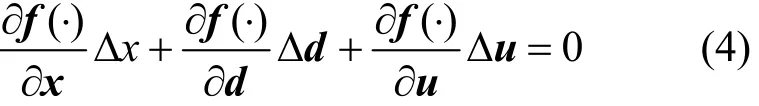
Adding Eqs. (3a), (3b) and (3c), we obtain

For non-active constraints, there is Lagrange multiplier μj=0. The non-active constraints can be removed from Eq. (5),

The steady-state operating point of the optimal design generally lies on the boundaries of some process constraints, which are active constraints gi(·)=0. Because these active constraints are “hard”, process variables should be restricted within them when process runs. Since some uncertainties may violate active constrains, the margins Δd must be added to the design variables∗d, then the operating point will moveinto the feasible region and there are proper distances between current operating point and active constraints,

where Δgiis the distance from the operating point to the ith active constraint, Δgi<0.
For active constraints, the Lagrange multipliers μi≥0. When the margins are added on the design variables, the economic back-off of the optimal design can be related to the distances between current operating point and active constraints,
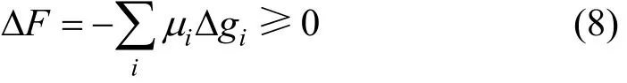
Therefore, when process design is completed and margins are added, the presence of Δgigives an opportunity for operation optimization. Adjusting the manipulation variables, we can move the operating point close to the process constraints to achieve more economic benefit, but the maximum economic benefit from operation optimization will not be larger than ΔF.
It can be seen that, if the margins Δd are added on the design variables, the operating point will locate within the boundaries of process constraints. The distances between current operating point and active constraints cause the economic back-off but provide the free space for operation optimization. After the process design is finished, we adjust the manipulation variables Δu through operation optimization to move the operating point close to the process constraints again to achieve more economic benefit, but the maximum economic benefit from operation optimization will not be larger than the economic back-off due to increasing margins. The maximum potential benefit from operation optimization is related to the design margins and can be used to represent the design margin of a chemical process.
3 STEADY-STATE OPTIMIZATION AND DYNAMIC OPTIMIZATION
The operation optimization of chemical process involves two aspects: steady-state optimization and dynamic optimization.
After process design is finished, design variables d remain unchanged and manipulation variables u can be adjusted as optimization variables. The steady-state optimization problem is described as
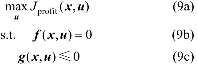
where Jprofitis a part of F, which is only relevant to manipulation variables u, namely economic benefit from operation optimization. It equals to the benefit from the product relevant to state variables minus the cost relevant to manipulation variables, that is

where csand cmare economic coefficient vectors of state variables and manipulation variables, respectively.
However, when process conditions change or disturbances occur, the process variables will vary with time under the effect of control system. Fig. 1 shows that the steady-state value is inside the range of constraint, but some of the dynamic values in transient process are outside the range of constraint. The dynamic optimization is necessary so that the process variables are inside the range of constraint in the whole dynamic process.
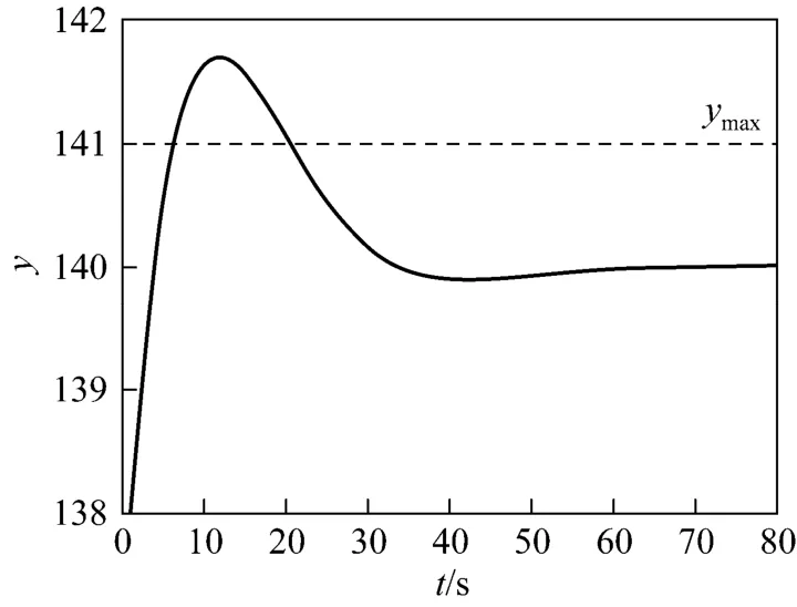
Figure 1 The relation between dynamic transient process and steady-state constraint
The dynamic optimization problem can be given by

where y represents the vector of controlled variables, χ0, u0, and y0are the nominal steady-state values of χ, u, and y, χdand χaare the vectors of differential variables and algebraic variables, respectively,v is the vector of disturbances in dynamic process, c is the vector of controller parameters, fd(·) and fa(·) are the vectors of the differential equations and algebraic equations in process model, respectively, ()⋅=fwhen the process is steady-state, h(·) is the vector of the output equations of controlled variables, fc(·) is the vector of controller model equations.
The dynamic equations of PID controller is described as

where,
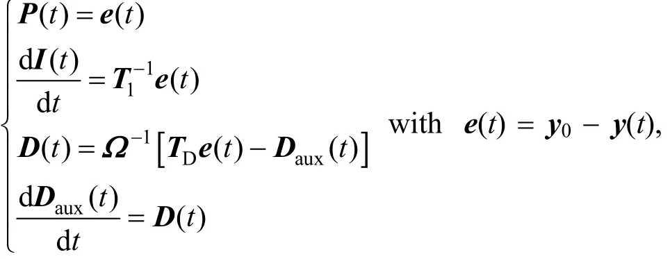
K is the diagonal matrix consisting of proportional gain, TIis the diagonal matrix consisting of reset time of the integral term, TDis the diagonal matrix consisting of rate time of the derivative term, Ω is the diagonal matrix consisting of bandwidth limit of the derivative term, e(t) is the error vector of controlled variables, P(t) is the vector of proportional term contribution for control output, I(t) is the vector of integral term contribution for control output, D(t) is the vector of derivative term contribution for control output, and Daux(t) is the vector of auxiliary variables for derivative term calculation.
In the dynamic optimization, the control performance of process control system can be embodied by integral absolute error (IAE), which consists of the weighed sum of integral absolute error of each conventional PID controller. Smaller IAE means better control performance, which is denoted as
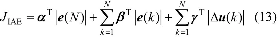
where α is the weighted coefficient vector of steadystate absolute error, β is the weighted coefficient vector of integral absolute error of dynamic transition process, and γ is the weighted coefficient vector of integral absolute control variation of dynamic transition process.
We used software gPROMS to solve the steadystate optimization and dynamic optimization. gPROMS is an equation-oriented dynamic process simulation and optimization software and can solve both steadystate and dynamic problems. gPROMS gives a direct access to the dynamic model providing differential equations and algebraic equations written in gPROMS language. The control vector parameterisation algorithm via single-shooting or multiple-shooting is used to transform the dynamic optimisation problem into a nonlinear programming problem. The nonlinear programming solver is the sequential quadratic programming algorithm. After the optimization variables and objective function are assigned, gPROMS can solve the dynamic optimization problem automatically.
4 OPERATION OPTIMIZATION AND CONTROL PERFORMANCE ANALYSIS
Steady-state optimization only involves the change between the steady-state starting operating point and the steady-state ending operating point, and it does not take the dynamic changes in transition process into consideration. However, there are various uncertain disturbances affecting the process plant, which cause frequent fluctuations of process variables. Some distances between the optimum operating point and process constraints must be reserved for the dynamic regulation of control system, which result in a back-off of economic benefit, as shown in Fig. 2. J0is the economic benefit of operation point A, which is the nominal operating point considering the margin. Because margins Δd are added on the design variables, the operating point A will locate within the boundaries of process constraints. J1is the economic benefit of operation point B of dynamic optimization, J2is the economic benefit of operation point C of steady-state optimization, and a distance may be reserved for operation point B and C. Thus we can find that J2>J1>J0obviously.
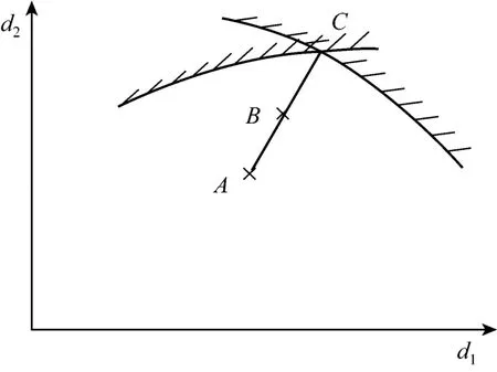
Figure 2 The operating point of dynamic optimization and steady-state optimizationA—nominal operating point considering margin; B—operating point of dynamic optimization; C—operating point of steady-state optimization
J2−J0that can be obtained through the steady-state operation optimization reflects the potential benefit and the whole margin of process plant, but it can not be fully achieved because of uncertain disturbances and control requirement. Only the benefit of dynamic operation optimization considering process disturbances and control system can be really achieved. Thus J1−J0is the really achievable benefit for profit, while J2−J1is the unachievable benefit paying for control and operation.
When the control system imposes dynamic regulation on process variables, the control action will consume design margins of process plant. The better control performance is requested, the more design margins are required. The overclaim for control performance will reduce the achievable benefit. However, if the design margins are sufficient, the fluctuations of process variables will be reduced by the control system, and the achievable benefit will increase. Thus we shouldinvestigate the interaction between design margins, control performance, and achievable benefit as a whole.
When we increase the margin for a design variable, steady-state optimization and dynamic optimization are carried out separately to calculate the potential benefit, achievable benefit, and corresponding control performance index IAE. Increasing the design margin continuously, we can draw the relation curve between design margin and potential benefit, achievable benefit, and IAE. We take the design margin as independent variable and the potential benefit, achievable benefit, and IAE as dependent variables. From the relation curve we can find the design bottleneck of current process plant.
In order to facilitate comparison and analysis, the design margin is denoted as relative percentage,
where dn, Δdn, and Mnare current values, the absolute margin to current value and the relative percentage margin of the nth design variable.
The achievable benefit ΔJ1=J1−J0(operation point B) and potential benefit ΔJ2=J2−J0(operation point C) are also denoted as relative percentage to the nominal benefit J0containing the margin (operation point A), that is

If the margin of a design variable increases a lot but it has little effect on the achievable benefit, we can conclude that the design margin is sufficient and there is no design bottleneck for operation optimization on the design variable. However, if the margin of a design variable increases a little but the achievable benefit increases a lot, it means that the design margin lacks and the design variable can be regarded as a design bottleneck for operation optimization. For design bottleneck, with a little margin added to the design variable, the achievable benefit will increase significantly.
Similarly, if the margin of a design variable increases a lot but it only leads to an unobvious change on the control performance, we can conclude that the design margin is sufficient for control and there is no bottleneck for control on the design variable. However, if the margin of a design variable increases only a little but it brings about great improvement on the control performance, it means that the design margin is insufficient for control and the design variable can be regarded as a design bottleneck for control. If we increase the design margin appropriately, the control performance will be improved significantly.
5 CASE STUDY
In this paper, the operation optimization and control performance analysis is based on a fluid catalytic cracking unit (FCCU) of refinery. Because the reactor is of great operating flexibility, the design margin is mainly concentrated on the regenerator.
Because of the catalyst circulation between the reactor and regenerator in FCCU, we consider the reactor and regenerator as a whole to discuss the relation between operation optimization and control performance. In this paper, the dynamic model of FCCU [1] is used.
In the operation optimization and control performance analysis, two design margins are considered, one for the regenerator catalyst inventory, and the other for the air flow rate of regenerator. For the steady-state optimization in Eq. (9) and the dynamic optimization in Eq. (11), the objective function is equal to the benefit of oil products minus the cost relevant to manipulation variables, optimization variables are mainly the reaction temperature of riser outlet and the flow rate of feed oil, and process constraints include production requirements and operating constraints, such as reaction temperature of riser outlet, mass fractions of product oils (diesel, gasoline and gas), temperature of regenerator, coke mass fraction of regenerated catalyst, oxygen mole fraction of flue gas, opening of slide valve, differential pressure on both sides of slide valve, and so on.
The dynamic model of process disturbances is given by where v0is the nominal value, v1, v2and v3are the amplitudes, ω1, ω2and ω3are the frequencies, ϕ1, ϕ2and ϕ3are the phases, for sinusoid variation, square change, and first-order inertial square change, respectively. T3is the time constant of first-order inertial square change.
For the FCCU reactor/regenerator system, we consider the following three regulatory control structures (RCS).
RCS1: the catalyst circulation rate controls the reaction temperature of riser outlet, and the air flow rate of regenerator is not a manipulation variable and remains constant.
RCS2: the catalyst circulation rate controls the reaction temperature of riser outlet, and the air flow rate of regenerator controls the oxygen mole fraction of flue gas.
RCS3: the catalyst circulation rate controls the reaction temperature of riser outlet, and the air flow rate of regenerator controls the temperature of regenerator.
Under the three control structures, with the increase of design margin, steady-state optimization and dynamic optimization are implemented separately to calculate the potential benefit, achievable benefit, and corresponding control performance index IAE. Increasing the design margin continuously, we can draw the relation curve, taking the design margin as independent variable and the potential benefit, achievablebenefit, and IAE as dependent variables.
Figure 3 shows the relation curves, with the design margin of air flow rate as independent variable. Under the three regulatory control structures, as the design margin of air flow rate increases, both potential benefit and achievable benefit increase accordingly, while IAE decreases in overall trend, meaning that the control effect is improved significantly. We can conclude that the air flow rate is a bottleneck design variable of FCCU for both operation optimization and control.
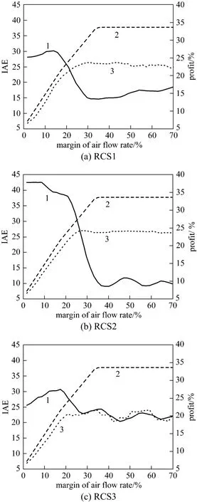
Figure 3 Relation curves of potential benefit, achievable benefit and control performance under three regulatory control structures with design margin of air flow rate as independent variable1—control performance; 2—potential benefit; 3—achievable benefit
In the initial segment of Fig. 3, there is no obvious difference between potential benefit and achievable benefit and the control performance is poor. We conclude that, for inadequate design margin, the control performance shows competitive relationship with the achievable benefit, and the improvement of economic benefit needs to reduce the control performance as expense. Within the range from 20% to 30% of independent variable, the difference between potential benefit and achievable benefit begins to surge and the control performance is improved significantly. It indicates that the control system consumes some design margin to improve the control performance but reduces the proportion of achievable benefit in the potential benefit; meanwhile the process fluctuations are reduced by control system, so the achievable benefit increases at last. Beyond the point 30% of independent variable, the achievable benefit remains unchanged substantially, and the control performance fluctuates within a small range. Beyond the range from 30% to 40%, the potential benefit is also unchanged. It shows that the design margin is sufficient so that the air flow rate is no longer a bottleneck variable for operation optimization and control now.
For the three regulatory control structures, RCS2 is superior to RCS1 and RCS1 is better than RCS3, but there is no large difference. With inadequate design margin, the improvement of economic benefit is at the expense of reduction of control performance, so RCS1 should be adopted. With sufficient design margin, RCS2 is favorable to meet the requirements of operation optimization and control performance simultaneously.
Figure 4 shows the relation curves with the design margin of regenerator catalyst inventory as independent variable. Under the three regulatory control structures, as the design margin of regenerator catalyst inventory increases, the potential benefit, achievable benefit and IAE do not change much. We conclude that the regenerator catalyst inventory is not a bottleneck design variable of FCCU for both operation optimization and control. For the achievable benefit, RCS2 is the highest, and RCS1 and RCS3 have little difference. For the control performance, RCS2 is superior to RCS1 and RCS1 is better than RCS3, so RCS2 should be adopted.
6 CONCLUSIONS
For chemical processes, a steady-state optimization was used to evaluate potential benefit, and a dynamic optimization was used to evaluate achievable benefit and corresponding control performance. With the analysis on how the margins of design variables influence economic benefit and control performance, the bottlenecks of process design could be found and appropriate control structure could be selected. The conclusions are as follows.

Figure 4 Relation curves of potential benefit, achievable benefit and control performance under three regulatory control structures with design margin of regenerator catalyst inventory as independent variable1—control performance; 2—potential benefit; 3—achievable benefit
(1) Based on the relation curves between design margin and potential benefit, achievable benefit, and control performance index IAE, the design bottleneck of current process plant could be found. If the margin of a design variable increases a lot but hardly influences the achievable benefit and control performance, the design variable is not a design bottleneck for operation optimization and control. Otherwise, it is a design bottleneck and needs to increase the margin.
(2) With inadequate design margin, there is a competitive relationship between control performance and achievable benefit, and the improvement of economic benefit is at the expense of reduction of control performance. With sufficient design margin, the conflict of margin requirement between control and operation optimization could be solved effectively, and the improvement of control performance will contribute to the promotion of achievable benefit.
(3) When the design margin changes, it may be necessary to adjust control system structure to satisfy the requirements of operation optimization and control performance simultaneously.
NOMENCLATURE
c vector of controller parameters
cs, cmeconomic coefficient vectors of state variables and manipulation variables
D vector of derivative term contribution for control output of PID controller
Dauxvector of auxiliary variables for derivative term calculation of PID controller
d vector of design variables
e errors vector of controlled variables
F objective function of optimal design
f vector of process model equations
fa, fdvectors of algebraic equations and differential equations in process model
fcvector of controller model equations
g vector of equations of process constraints
h vector of output equations of controlled variables
I vector of integral term contribution for control output of PID controller
Jprofitobjective function of operation optimization
K diagonal matrix consisting of proportional gain of PID controller
L Lagrange function
P vector of proportional term contribution for control output of PID controller
TIdiagonal matrix consisting of reset time of the integral term of PID controller
TDdiagonal matrix consisting of rate time of the derivative term of PID controller
u vector of control variables
v vector of disturbances
χ vector of state variables
χa, χdvector of algebraic variables, differential variables
y vector of controlled variables
α, β, γ weighted coefficient vectors of steady-state absolute error, integral absolute error, integral absolute control variation
Δ variation
λ Lagrange multiplier vector of equality constraints
μ Lagrange multiplier vector of inequality constraints
Ω diagonal matrix consisting of bandwidth limit of the derivative term
Superscripts
T matrix transposition
* optimal design
NOMENCLATURE
i active constraints
j non-active constraints
m manipulation variable
s state variable
0 nominal steady-state value
REFERENCES
1 Xu, F., Luo, X., “Margin analysis and control design of FCCU regenerator based on dynamic optimization (I) Mathematical description of dynamic optimization”, CIESC Journal, 60 (3), 675-682 (2009). (in Chinese)
2 Xu, F., Luo, X., “Margin analysis and control design of FCCU regenerator based on dynamic optimization (II) Solution and result analysis”, CIESC Journal, 60 (3), 683-690 (2009). (in Chinese)
3 Xu, F., Luo, X., “Analysis of air rate margin in FCCU regenerator based on dynamic model”, Journal of Chemical Industry and Engineering, 59 (1), 126-134 (2008). (in Chinese)
4 Xu, F., Luo, X., “Manipulation margin and control performance analysis of chemical process under advanced process control”, CIESC Journal, 63 (3), 881-886 (2012). (in Chinese)
5 Kuhlmann, A., Bogle, I., “Controllability evaluation for nonminimum phase-processes with multiplicity”, AIChE J, 47 (11), 2627-2631 (2001).
6 Figueroa, J.L., Bahri, P.A., Bandoni, J.A., Romagnoli, J.A., “Economic impact of disturbance and uncertain parameters in chemical processes—A dynamic back-off analysis”, Computers and Chemical Engineering, 20 (4), 453-461 (1996).
7 Soliman, M., Swartz, C., Baker, R., “A mixed-integer formulation for back-off under constrained predictive control”, Computers and Chemical Engineering, 32 (10), 2409-2419 (2008).
8 Li, Z., Hua, B., “Flexible synthesis of heat exchanger networks for multi-period operation”, Journal of Chemical Engineering of Chinese Universities, 13 (3), 252-258 (1999). (in Chinese)
9 Xu, Q., Chen, B., He, X., “Flexible synthesis in chemical processing systems”, Journal of Tsinghua University, 41 (6), 44-47 (2001). (in Chinese)
10 Karafyllis, I., Kokossis, A., “On a new measure for the integration of process design and control: The disturbance resiliency index”, Chemical Engineering Science, 57 (5), 873-886 (2002).
11 Bansal, V., Perkins, J.D., Pistikopoulos, E.N., “A case study in simultaneous design and control using rigorous, mixed-integer dynamic optimization models”, Industrial & Engineering Chemistry Research, 41 (4), 760-778 (2002).
12 Ulasa, S., Diwekar, U.M., “Integrating product and process design with optimal control: A case study of solvent recycling”, Chemical Engineering Science, 61 (6), 2001-2009 (2006).
13 Miranda, M., Reneaume, J. M., Meyer, X., Meyer, M., Szigeti, F.,“Integrating process design and control: An application of optimal control to chemical processes”, Chemical Engineering and Processing, 47 (11), 2004-2018 (2008).
14 Sakizlis, V., Perkins, J. D., Pistikopoulos, E. N., “Parametric controllers in simultaneous process and control design optimization”, Industrial & Engineering Chemistry Research, 42 (20), 4545-4563 (2003).
15 Chawankul, N., Budman1, H., Douglas, P.L., “The integration of design and control: IMC control and robustness”, Computers and Chemical Engineering, 29 (2), 261-271 (2005).
16 Bansal, V., Sakizlis, V., Ross, R., Perkins, J.D., Pistikopoulos, E.N.,“New algorithms for mixed integer dynamic optimization”, Computers and Chemical Engineering, 27 (5), 647-668 (2003).
17 Lu, X. J., Li, H., Yuan, X., “PSO-based intelligent integration of design and control for one kind of curing process”, Journal of Process Control, 20 (10), 1116-1125 (2010).
18 Ricardez-Sandoval, L.A., Budman, H.M., Douglas, P.L., “Application of robust control tools to the simultaneous design and control of dynamic systems”, Industrial & Engineering Chemistry Research, 48 (2), 801-813 (2009).
19 Ricardez-Sandoval, L.A., Budman, H.M., Douglas, P.L., “Simultaneous design and control: A new approach and comparisons with existing methodologies”, Industrial & Engineering Chemistry Research, 49 (6), 2822-2833 (2010).
20 Ricardez-Sandoval, L.A., Douglas, P.L., Budman, H.M., “A methodology for the simultaneous design and control of large-scale systems under process parameter uncertainty”, Computers and Chemical Engineering, 35 (2), 307-318 (2011).
21 Sakizlis, V., Perkins, J.D., Pistikopoulos, E.N., “Recent advances in optimization based simultaneous process and control design”, Computers and Chemical Engineering, 28 (10), 2069-2086 (2004).
22 Asteasuain, M., Brandolin, A., Sarmoria, C., Bandoni, A., “Simultaneous design and control of a semibatch styrene polymerization reactor”, Industrial & Engineering Chemistry Research, 43 (17), 5233-5247 (2004).
23 Asteasuain, M., Sarmoria, C., Brandolin, A., Bandoni, A., “Integration of control aspects and uncertainty in the process design of polymerization reactors”, Chemical Engineering Journal, 131 (1-3), 135-144 (2007).
24 Flores-Tlacuahuac, A., Biegler, L. T., “Integrated control and process design during optimal polymer grade transition operations”, Computers and Chemical Engineering, 32 (11), 2823-2837 (2008).
25 Grosch, R., Monnigmann, M., Marquardt, W., “Integrated design and control for robust performance: Application to an MSMPR crystallizer”, Journal of Process Control, 18 (2), 173-188 (2008).
10.1016/S1004-9541(14)60010-0
2013-08-15, accepted 2013-09-10.
* Supported by the National Natural Science Foundation of China (21006127), the National Basic Research Program of China (2012CB720500), and the Science Foundation of China University of Petroleum (KYJJ2012-05-28).
** To whom correspondence should be addressed. E-mail: xufengfxzt@sohu.com
 Chinese Journal of Chemical Engineering2014年1期
- Chinese Journal of Chemical Engineering的其它文章
- Photocatalytical Inactivation of Enterococcus faecalis from Water Using Functional Materials Based on Natural Zeolite and Titanium Dioxide*
- A Group Contribution Method for the Correlation of Static Dielectric Constant of Ionic Liquids*
- Measurement and Modeling for the Solubility of Hydrogen Sulfide in Primene JM-T*
- Enhancing Structural Stability and Pervaporation Performance of Composite Membranes by Coating Gelatin onto Hydrophilically Modified Support Layer*
- Kinetic Study on Extraction of Red Pepper Seed Oil with Supercritical
- Interaction Analysis and Decomposition Principle for Control Structure Design of Large-scale Systems*