
Photochemical Process Modeling and Analysis of Ozone Generation
2014-07-18 12:09WANGBing王冰QIUTong邱彤andCHENBingzhen陈丙珍DepartmentofChemicalEngineeringTsinghuaUniversityBeijing100084China
关键词:王冰
WANG Bing (王冰), QIU Tong (邱彤) and CHEN Bingzhen (陈丙珍)*Department of Chemical Engineering, Tsinghua University, Beijing 100084, China
Photochemical Process Modeling and Analysis of Ozone Generation
WANG Bing (王冰), QIU Tong (邱彤) and CHEN Bingzhen (陈丙珍)*
Department of Chemical Engineering, Tsinghua University, Beijing 100084, China
Air pollution in modern city and industrial zones has become a serious public concern in recent years in China. Significance of air quality assessment and emission control strategy design is increasing. Most studies in China focus on particulate matter (PM), especially PM2.5, while few account for photochemical secondary air pollutions represented by ozone (O3). In this paper, a procedure for air quality simulation with comprehensive air quality model with extensions (CAMx) is demonstrated for studying the photochemical process and ozone generation in the troposphere. As a case study, the CAMx photochemical grid model is used to model ozone over southern part of Beijing city in winter, 2011. The input parameters to CAMx include emission sources, meteorology field data, terrain definition, photolysis status, initial and boundary conditions. The simulation results are verified by theoretical analysis of the ozone generation tendency. The simulated variation tendency of domain-wide average value of hourly ozone concentration coincides reasonably well with the theoretical analysis on the atmospheric photochemical process, demonstrating the effectiveness of the procedure. An integrated model system that cooperates with CAMx will be established in our future work.
comprehensive air quality model with extensions, multi-scale, ozone, air quality modeling, photochemical
1 INTRODUCTION
Ground-level ozone (O3) is primarily produced from its precursors of NOχ(NO and NO2) and volatile organic compounds (VOC) by complex photochemical reactions in sunlight. Accumulation of ozone at ground level is influenced by physical and chemical processes and by meteorological conditions, which is potentially more harmful than its precursors [1]. The elevated concentration of O3at ground level is of particular concern, since it is known to have adverse effects on lung function and irritate the respiratory system. Exposure to ground level ozone and its precursor pollutants is linked to premature death, bronchitis, asthma, heart attack and other problems. The current state and progress in measurement, analysis and modeling of ozone precursors, photochemical behavior, and transport processes in troposphere have been reviewed [2-6]. Photochemical models are frequently employed to predict hourly ozone variations and help to establish cost-effective methods of reducing ambient ozone to control, in particular, the emissions of VOC and NOχfrom primary sources.
Beijing is one of the largest cities in the world with population over 19.61 million (2010) and covering 16807.8 km2. During the last two decades, Beijing has achieved its intensive urbanization and economic development, which leads to serious air quality problems characterized by elevated concentration of particulate matters and sulfur dioxide. The increase in coal, traffic and energy consumption is to be blamed for the increasingly serious air quality problem [7-9]. However, the majority of attention on air pollution focuses on traditional pollutants such as particulate matter and sulfur dioxide, while only limited studies have concentrated on photochemical ozone pollution [10]. Unfortunately, Beijing suffered obvious ozone polluting years ago. In June-July 2005 daily maximum ozone concentrations exceeded 236 μg·m−3for 13 days within 39 days with the peak hourly value of 561 μg·m−3[11]. Since the formation of O3is a complex process, involving various chemical and physical processes, it is of great significance to establish numerical models in order to link emissions and ambient concentrations based on specific chemical and physical processes and develop corresponding tool in analyzing detailed process for O3formation.
Most air quality models are developed based on transfer and diffusion process of pollutants in atmospheric processes. Some simulation work implements models as a “black box” to obtain temporal and spatial distribution of O3or other pollutants, and the model is mainly validated by comparing predicted and observed data [12, 13]. Further study emphasizes typical summertime O3episode over the Beijing area and uses the community multi-scale air quality (CMAQ) modeling system to simulate and analyze the observed data. Results show that ozone formation in urban area is VOC-limited but it changes to NOχ-limited in urban downwind area [14]. The influence of meteorological parameters has been analyzed in ozone formation in Kaohsiung, Taiwan using CAMx version 2.0 with an ozone-NOχ-VOC sensitivity analysis [15]. A systematic evaluation of ozone control strategies in Hong Kong is developed using the sparse matrix operating kernel emissions model (SMOKE version 2.4) for emission processing, the fifth-generation NCAR/Penn State mesoscale model (MM5) version 3.7 for meteorology, and CAMx v5.10 for chemical transport modeling to build a cooperating model system [16].
In this paper, a procedure for using an air quality model of CAMx is presented to study the photochemical process and ozone generation in the troposphere. As a case study, CAMx v5.40 is used to establish amodel system for the simulation of ozone formation process in troposphere with particular meteorology and emission data for Beijing domain and some assumptions are employed in preparing emissions and other input parameters. Model performance is compared with ozone formation theory.
2 PROCEEDURE DESCRIPTION
2.1 Introduction of core model CAMx
The comprehensive air quality model with extensions, CAMx in short, is developed by ENVIRON Corporation, (http://www.camx.com/) USA. Model CAMx simulates the emission, dispersion, chemical reaction, and removal of pollutants in the troposphere by solving the pollutant continuity equation for each chemical species on a system of nested three-dimensional grids [Eq. (A1)], and the continuity equations of the processes described above are shown in Appendix, Eqs. (A2)-(A9). The six generation of carbon bound photochemical mechanism (CB06) is used for gas phase chemistry, along with the Euler-Backward iterative (EBI) chemical kinetics solver, while the area preserving flux-form advection solver of BOTT (1989) is employed in CAMx as horizontal advection solver and “K-theory” is used in the vertical diffusion solver. To improve the computational efficiency, parallel processing, including OpenMP (OMP, shared memory parallel processing) and message passing interface (distributed memory parallel processing), is also supported in CAMx.
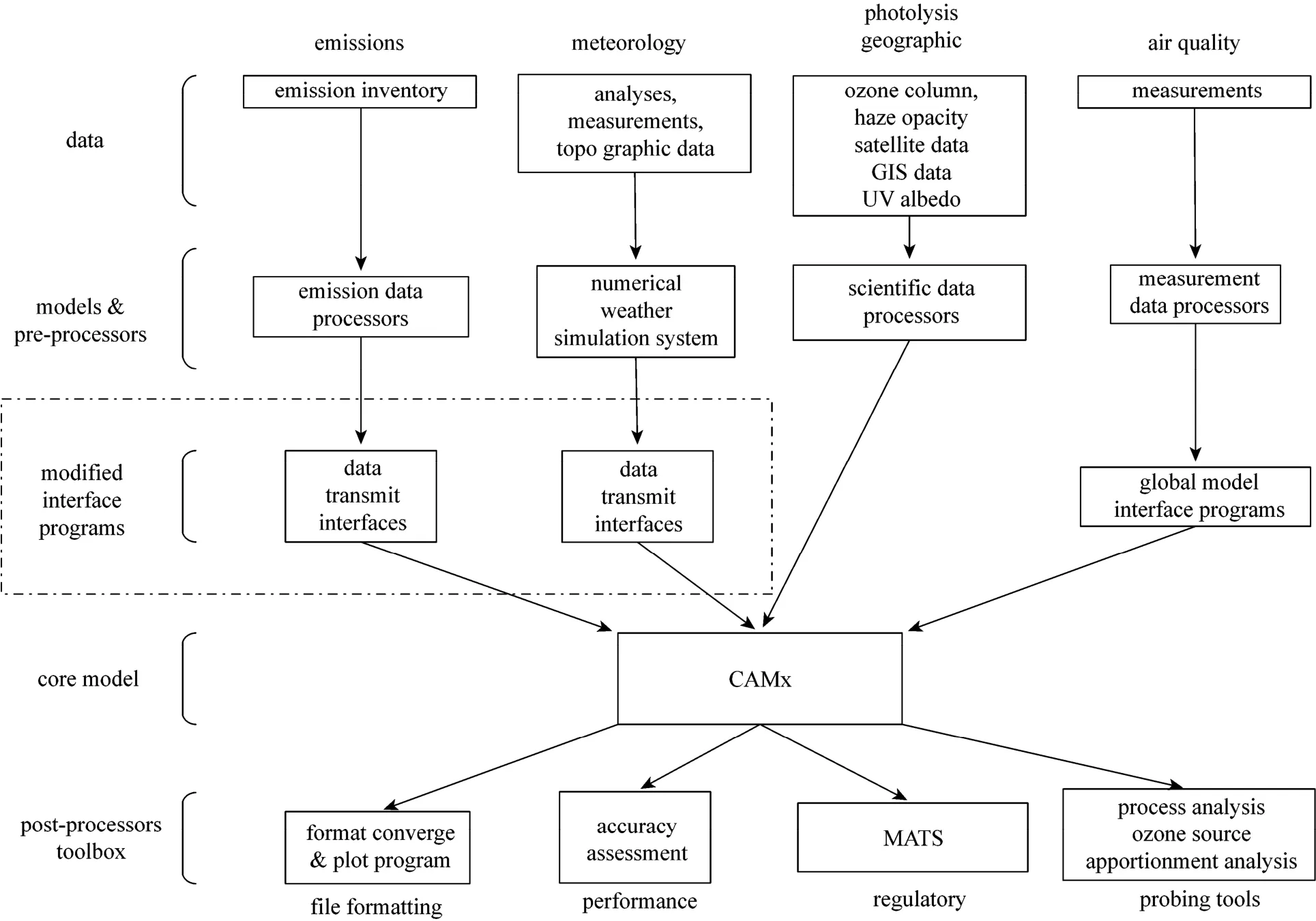
Figure 1 Schematic diagram of the procedure for using CAMx to simulate photochemical process and ozone generation in the troposphere with secondary developed interface programs (in dot-dash line) GIS—geographic information system; MATS—modeled attainment test software
2.2 Description of model system
CAMx is a specific core model dealing with photochemical process simulation and result analyses. To achieve the atmospheric simulation, CAMx multiscale model needs to cooperate with various third-party visualization software, meteorological models and emission processors, with necessary interface programs and post-processors. Fig. 1 is a schematic diagram of the CAMx modeling system (visit http://www.camx.com/files/camxusersguide_v5-40.pdf for details). The core model of CAMx requires four primary data sources including emissions, meteorology, photolysis and geographic air quality observation data. Independent models for emission data process, meteorological field prediction, ozone column preparation and geographic information system are introduced to provide the input data with specific interfaces provided by CAMx. The whole model system constitutes a platform to simulate the photochemical process in the atmosphere precisely. CAMx also provide usefultoolbox of post-analysis, such as ozone source apportionment technology (OSAT), particulate source apportionment technology (PSAT), decoupled direct method (DDM), process analysis (PA) and reactive racers (RTRAC). These extensions help to evaluate the model performance in our future work. Secondary development of interface programs between CAMx core and its pre-processors is implemented based on original interfaces of the model. In this work, we focus on the procedure of photochemical process simulation, and the implement of this analysis will be demonstrated in our future work.
3 CASE STUDY
3.1 Model domain
The CAMx core model is employed and tested with a case study based on Beijing domain. Fig. 2 shows the model domain and master grid settings. Target area (center of the Beijing city) is darkened. Here the Universal Transverse Mercator Grid System (UTM) is used to locate the domain area, whose coordinate of origin point (south-east corner) is UTM 50S, 373.13 km East and 4377.2 km North (50 indicate that the domain is located in the 50th zone whose longitude is 114°E-120°E, S indicate that the domain is in the latitude region of 32°N-40°N; the following two distance values are UTM-E and UTM-N coordinates, which describe the specific location of the origin point in the 50S zone). The full horizontal domain is 105 km long and 56 km wide and contains 105×56 horizontal coarse grid cells of 1 km×1 km. Since the computational accuracy of the high density coarse grid is sufficient for air quality models, there is no need to set fine nested grid to increase the precision. Sixteen vertical layers are installed with the layer interfaces at 30, 70, 100, 150, 300, 450, 600, 750, 1050, 1400, 1800, 2500, 4000, 6500, 9000 and 14000 m. The model domain covers 12 districts of Beijing city, 8 of which constitute center city (darkened area), while the other 4 districts form the surrounding area.
3.2 Meteorological conditions
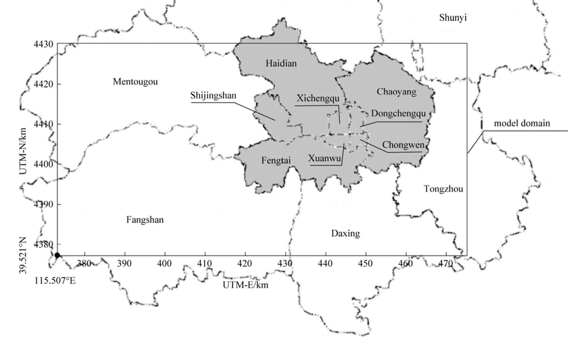
Figure 2 Beijing domain and master grid boundary (darken area: center of Beijing city; coordinate of southeast corner: 115.507°E, 39.521°N; UTM-E and UTM-N is the specific coordinate inside the certain 50s zone)
The two-day simulation requires hourly data of meteorological conditions, such as wind field (speed and direction), temperature, pressure, relative humidity, and period of sunshine. These scatter data collected from 30 automatic meteorological observing stations governed by Beijing Meteorological Bureau are plotted and interpolated to grid using Golden software Surfer (Version 10) hour by hour, then a self-compiled Fortran program is introduced to combine these data in certain order required by CAMx v5.40. The horizontal wind field at each grid node is expressed as perpendicular components (u, v) by the self-compiled FORTRAN program. Some assumptions are employed to describe the meteorological field. The vertical diffusivity (m2·s−1), which governs the vertical transport rate of gas components, is generated by a CAMxpre-processor program to apply the minimum vertical diffusivity values to layers below 100 m based on input landuse grid. The landuse parameter shows weighted average of landuse for each cell. Table 1 lists the minimum value of vertical diffusivity based on average weight of landuse type. The vertical diffusivity is also influenced by atmospheric stability [17]. Furthermore, with the atmospheric stability throughout daytime and nighttime, the vertical diffusivity value should be time-various. Since the photochemical processes only occur during the daytime with sufficient sunlight and the ground-level ozone is barely present in the night, it is reasonable to assume the vertical diffusivity to be time-invariant and equal to the daytime values.
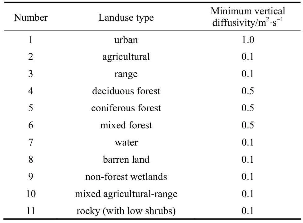
Table 1 Eleven types of landuse and corresponding minimum vertical diffusivity values
3.3 Initial and boundary conditions
CAMx requires three-dimensional field of initial concentration for simulation on the master grid, and the initial condition input file contains concentration of each chemical species in each master grid cell. There is no need to provide initial concentration data for fine nested grid cells, since CAMx will interpolate all master grid initial conditions to every fine nested grid at the start of the simulation whether the fine nest grid is established or not. The initial concentration input file is generated based on a time and spaceinvariant concentration file, named as TOPCON, which contains individual species for the entire domain. The ozone concentration in our TOPCON is set to 60 μg·m−3according to [15]. Lateral boundary conditions determine the exchange of chemical components between the model domain and surrounding area. Boundary concentration can be either time-invariant or time-variant. In this simulation, lacking of observation data, the boundary concentration is assumed time-invariant with a small range of randomness.
CAMx defines the “lower bound” values for those species not considered in initial and boundary conditions. The “lower bound” value is specified in the chemical parameter files released with CAMx source code.
3.4 Pointed and gridded emissions
CAMx supports two input emissions: elevated point source and gridded emissions. Elevated point source input file contains stack parameters and emission rates for all elevated point sources and emitted species. Gridded emission file is a combination of various types of emission sources, such as biogenic source, mobile source, anthropogenic sources, non-road source, residential sources, non-point industrial sources and natural sources. Mobile emissions for this simulation are developed based on the study of [18, 19]. In order to simplify the generation of emission input, the vehicular emissions, NOχand VOCs, are assumed to be time-invariant, with higher value from 7:00 to 20:00 and lower value between 20:00 and 7:00 the next day. Biogenic emissions are prepared on account of biogenic emission inventory [20]. The total gridded emission input is generated based on previous research [21], giving the daily temporal distribution of ozone and NOχconcentration in August, 2006. Since this simulation is for February 2011, we follow the daily concentration variation tendency of NOχand other ozone precursors and import proper factors to reduce the release levels of these emissions from August. The released amount of other precursors remains stable throughout the year [22]. Industrial emissions in the model domain are mainly assembled in Yanshan Petrochemical Plants in Fangshan district. The industrial emission is roughly determined according to the Handbook of Industrial Pollution Source Emission Coefficient during the First China Pollution Source Census (http://cpsc.mep.gov.cn/, Chinese). Elevated point emission defines the single, elevated emission source.
In this simulation, elevated point source emissions are assumed by choosing 150 point sources in the domain area with a dense point source distribution in the center city (darken area in Fig. 2) and a sparse distribution in the four surrounding districts. CAMx requires the point source file to provide specified time-resolved emission rates and stack parameters for each individual source. The input point source emission rates and stack parameters are generated based on the CAMx official testing case (http://www.camx.com/download/camx-test-case.aspx) using a self-compiled FORTRAN program.
4 RESULTS AND DISCUSSION
The model is processed on a HP workstation with 4 CPU nodes expanding to 8 threads using OMP shared memory paralleling computing, with 6 threads employed for the calculation. A 48-hour simulation covering 105×56 master grids takes 2 h. Fig. 3 shows the domain-wide average value of hourly ozone concentration (c). The variation tendency is the same as that in literature [15]. With the initial conditions, the ozone concentration variation tendency agrees with the photochemical process of ozone generation.Photochemical process starts when the two main precursors for ozone formation, VOC and NOχ, are both present in the atmosphere with sufficient sunlight, then ozone is generated through complex photochemical reactions. As ozone generates, primary pollutants NOχand VOCs are consumed. These ozone precursors not only help to generate ozone but also consume ozone, and the generation speed versus consuming speed is determined by the concentration of NOχ. Before the concentration of NO2descends to a critical value, the ozone concentration keeps increasing. In Beijing, the morning peak is serious and a large number of vehicles produce masses of NOχand VOCs during 7:00 to 9:00 am, which helps to generate large amount of secondary photochemical pollutants, including ozone. That explains the two peaks of ozone concentration around 10:00 am. In the afternoon, as the sunlight intensity decreases, the generation of ozone is less and the concentration of ozone keeps decreasing through the night.
Figure 4 shows the average ozone concentration of the entire domain at 10:00, 14:00 and 18:00 on Feb. 21, 2011 with the wind field. Fig. 5 shows that at 10:00, 14:00 and 20:00 the next day. Areas with O3concentration above 160 μg·m−3, 180 μg·m−3and 200 μg·m−3are marked with contour line individually. On the first day, about three quarters of the domain region are covered with O3with concentration higher than 160 μg·m−3, while the hot spot region with O3concentration exceeding 200 μg·m−3locates northeast of the model domain, covering a relatively smaller area, and the hot spot region reduces with time and disappears at 18:00. On the next day, a large area with O3concentration exceeding 200 μg·m−3appears on Fig. 5 (a), covering almost one third of the total model domain. Though the area of the hot spot region decreases with time, it does not disappear and remains about one fifth of the total domain region at 20:00 in the night.
In Fig. 4 (a), it is reasonable for the hot spot to appear at 10:00 in the northeast and cover a relatively small area because it covers the center of Beijing, with a mass of vehicles and buildings as well as over 60% of the population. A ground level of high pressure center is located to the south of the hot spot region, which leads to complex wind field in the hot spot region, making pollutant dilution difficult. In Fig. 5 (a), a recognizable relatively high pressure system is located in the middle of the model domain, making wind field complex to some extent and slowing down the pollution dilution. Besides, according to Fig. 3, on Feb. 22, ground level ozone starts to accumulate at a concentration of approximately 140 μg·m−3at the initial time, which is 17 μg·m−3higher than the previous day. With relatively lower wind speed on Feb. 22 compared with that on Feb. 21, the appearance of larger area of O3concentration above 200 μg·m−3is reasonable.
Influences of wind are prominent in Fig. 5 (c). Since the wind speed at 20:00 is relatively lower than that at 14:00 [Fig. 5 (b)] and 10:00 [Fig. 5 (a)], judging from the length of wind vectors, the transmission of ozone and other pollutants by wind is weaken, so the dilution of ozone is more difficult than the previous day. All of these effects result in the large area of ozone with concentration above 200 μg·m−3.
Notably, low wind speed and sufficient precursors and sunlight lead to high ozone concentration. The influences of initial conditions at the start of each simulation day are roughly analyzed and proved on high ozone distribution. In summary, no single meteorological parameter suffices to explain the high O3concentration. As far as the model could describe, it is a comprehensive influence of meteorological parameters, initial and boundary conditions as well as emissions sources that determines the formation of ground level ozone. The accuracy of CAMx is also influenced by these internal and external characters. Internal characters of CAMx model such as the built-in parameters of photochemical kinetics and numerical method influence the model accuracy. External characters are extensive input data containing emission sources, meteorological data, landuse, photolysis parameters including UV albedo information described in Fig. 1. The model accuracy is usually examined by observed data. Sensitivity analysis and process analysis are necessary and effective methods to improve the model performance and adjust model parameters. Model assessment based on sensitivity analysis shows various influences of different model parameters that affect model performance and helps to find key factors. We make adjustment under the guidance of sensitivity analysis and process analysis as well as the statistical analysis based on observed data. Furthermore, since the extensive input data introduce considerable uncertainty, which is quite difficult for researchers to take into consideration, reasonable simplification is unavoidable, and the research on uncertainty analysis is needed.

Figure 3 Evaluated domain-wide average value of hourly ozone concentration in the 48-hour simulation
5 CONCLUSIONS
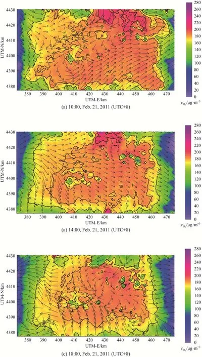
Figure 4 Average hourly ozone concentration estimated by CAMx at 10:00 (a), 14:00 (b) and 18:00 (c) on Feb. 21, 2011 with wind field
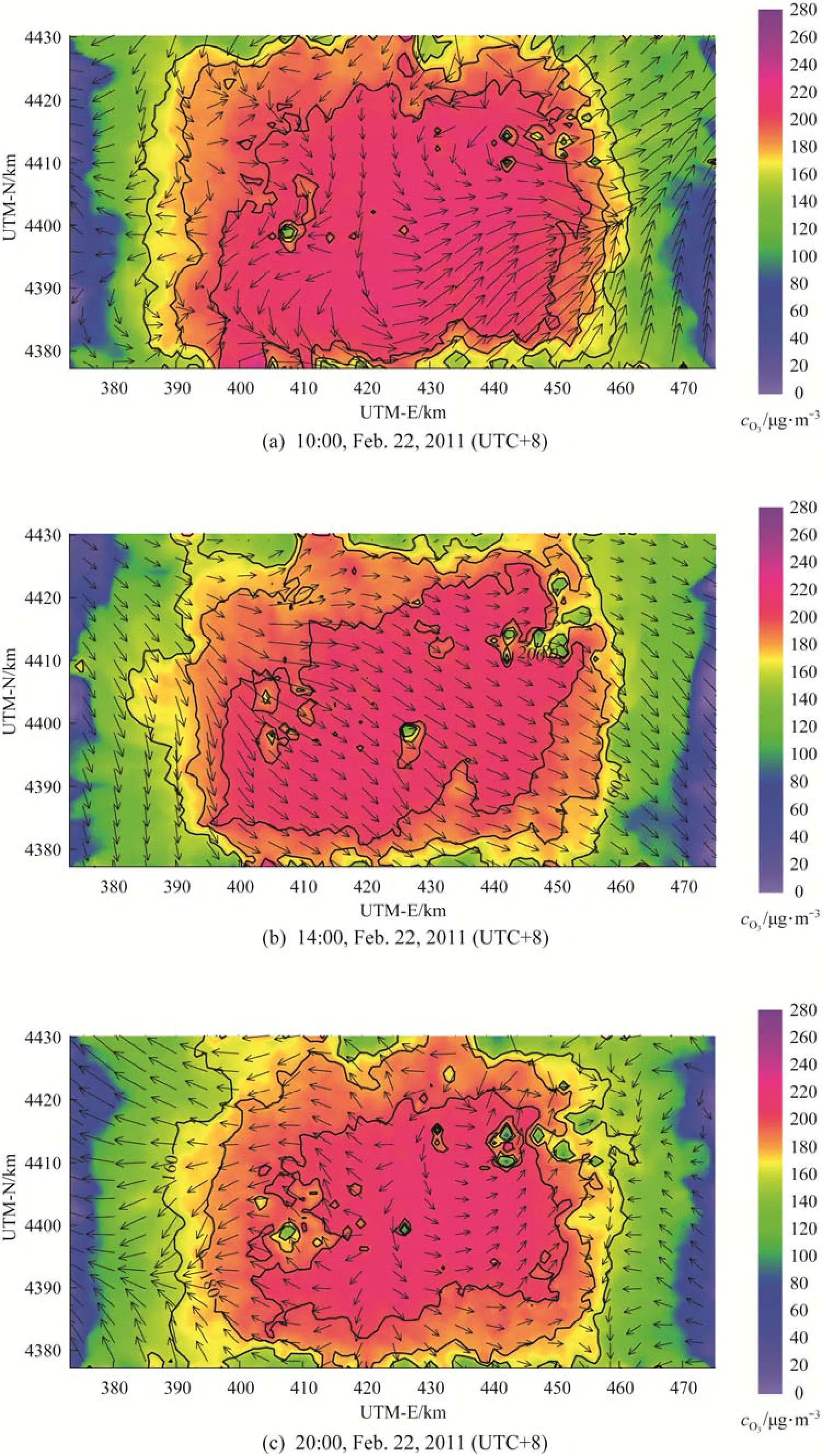
Figure 5 Average hourly ozone concentration estimated by CAMx at 10:00 (a), 14:00 (b) and 20:00 (c) on Feb. 22, 2011 with wind field
A procedure of the implementation of CAMx to study the photochemical process and ozone generation in the troposphere was illustrated in this paper. As a case study, photochemical modeling and ozone generation analysis were performed for Beijing city in winter,2011. The hourly domain-wide average ozone concentrations coincide reasonably well with the atmospheric photochemical process theory. The assessment reveals that initial conditions play a crucial role in determining the ozone distribution. Effects of meteorological parameters, wind fields in particular, indicate that the local high pressure system with ground obstacle could lead to chaotic wind direction and block the dispersion and dilution of ozone, maintaining an elevated ozone concentration region.
6 FUTURE WORK
Although this paper has demonstrated a procedure to implement an air quality model of CAMx to study the photochemical process and ozone generation in the troposphere, a lot of work is needed in the future. Atmospheric photochemical process simulation requires extensive input data covering emission inventories, meteorological fields, photolysis, geographic information and observation. Each of these input aspects is originally an independent research field and requires careful study to acquire enough accuracy and reliability, which means massive teamwork. When the input data are collected or prepared, a rectification process is needed to enhance their reliability. Input data are divided into two parts based on their measurability. Measurable data, such as wind speed, temperature, humidity, pressure, emissions, and land covers, are collected with certain redundancy in order to get rid of random error and estimate unmeasurable process variables. Gross errors are also detected and eliminated in the process of data reconciliation [23]. Unmeasurable data essential for modeling are collected from the achievement of predecessors, such as photochemical kinetics of carbon bond theory and vertical diffusivity coefficient [15].
As shown in Fig. 1, CAMx deals with extensive input data and provide sufficient toolboxes to analyze the results and photochemical process, including result conversion and plotting, process analysis, sensitivity analysis, ozone source apportionment analysis, etc.
To improve the model accuracy and reliability, systematic uncertainty analyses are also required to improve and evaluate model performance, so that we can find the most influential aspect and dealing with it using specific method or measurements.
REFERENCES
1 Swackhamer, D.L., “Rethinking the ozone problem in urban and regional air pollution”, J. Aerosol. Sci., 24 (7), 977-978 (1993).
2 Sillman, S., “The relation between ozone, NOχand hydrocarbons in urban and polluted rural environments”, Atmos. Environ., 33 (12), 1821-1845 (1999).
3 Hidy, G., “Ozone process insights from field experiments—part I: Overview”, Atmos. Environ., 34(12-14), 2001-2022 (2000).
4 Blanchard, C., “Ozone process insights from field experiments—Part III: Extent of reaction and ozone formation”, Atmos. Environ., 34 (12-14), 2035-2043 (2000).
5 Trainer, M., Parrish, D.D., Goldan, P.D., Roberts, J., Fehsenfeld, F.C.,“Review of observation-based analysis of the regional factors influencing ozone concentrations”, Atmos. Environ., 34 (12-14), 2045-2061 (2000).
6 Russell, A., “NARSTO critical review of photochemical models and modeling”, Atmos. Environ., 34 (12-14), 2283-2324 (2000).
7 Yang, F., Tan, J., Zhao, Q., Du, Z., He, K., Ma, Y., Duan, F., Chen, G., Zhao, Q., “Characteristics of PM2.5 speciation in representative megacities and across China”, Atmos. Chem. Phys., 11 (11), 5207-5219 (2011).
8 Wang, Y., Zhuang, G.S., Tang, A.H., Yuan, H., Sun, Y.L., Chen, S.A., Zheng, A.H., “The ion chemistry and the source of PM2.5 aerosol in Beijing”, Atmos. Environ., 39 (21), 3771-3784 (2005).
9 Molina, M.J., Molina, L.T., “Megacities and atmospheric pollution”, J Air Waste Manag Assoc, 54 (6), 644-680 (2004).
10 Hao, J.M., Wang, L.T., Li, L., Hu, J.N., Yu, X.C., “Air pollutants contribution and control strategies of energy-use related sources in Beijing”, Sci. China Ser. D-Earth Sci., 48, 138-146 (2005).
11 Hao, J., Wang, L., “Improving urban air quality in China: Beijing case study”, J Air Waste Manag Assoc, 55 (9), 1298-1305 (2005).
12 Shao, M., Tang, X., Zhang, Y., Li, W., “City clusters in China: Air and surface water pollution”, Front. Ecol. Environ., 4 (7), 353-361 (2006).
13 Smyth, S.C., Jiang, W., Yin, D., Roth, H., Giroux, É., “Evaluation of CMAQ O3and PM2.5 performance using Pacific 2001 measurement data”, Atmos. Environ., 40 (15), 2735-2749 (2006).
14 Xu, J., Zhang, Y., Fu, J.S., Zheng, S., Wang, W., “Process analysis of typical summertime ozone episodes over the Beijing area”, Sci Total Environ, 399 (1-3), 147-157 (2008).
15 Chen, K.S., Ho, Y.T., Lai, C.H., Chou, Y.M., “Photochemical modeling and analysis of meteorological parameters during ozone episodes in Kaohsiung, Taiwan”, Atmos. Environ., 37 (13), 1811-1823 (2003).
16 Li, Y., Lau, A.K.H., Fung, J.C.H., Ma, H., Tse, Y.Y., “Systematic evaluation of ozone control policies using an Ozone Source Apportionment method”, Atmos. Environ., 76, 136-146 (2013).
17 Steffens, J.T., Heist, D.K., Perry, S.G., Zhang, K.M., “Modeling the effects of a solid barrier on pollutant dispersion under various atmospheric stability conditions”, Atmos. Environ., 69, 76-85 (2013).
18 Lang, J., Cheng, S., Wei, W., Zhou, Y., Wei, X., Chen, D., “A study on the trends of vehicular emissions in the Beijing-Tianjin-Hebei (BTH) region, China”, Atmos. Environ., 62, 605-614 (2012).
19 Cai, H., Xie, S., “Estimation of vehicular emission inventories in China from 1980 to 2005”, Atmos. Environ, 41 (39), 8963-8979 (2007).
20 Wang, Z.H., Bai, Y.H., Zhang, S.Y., “A biogenic volatile organic compounds emission inventory for Beijing”, Atmos. Environ., 37 (27), 3771-3782 (2003).
21 Tang, X.A., Wang, Z.F., Zhu, J.A., Gbaguidi, A.E., Wu, Q.Z., Li, J., Zhu, T., “Sensitivity of ozone to precursor emissions in urban Beijing with a Monte Carlo scheme”, Atmos. Environ., 44 (31), 3833-3842 (2010).
22 Nopmongcol, U., Koo, B., Tai, E., Jung, J., Piyachaturawat, P., Emery, C., Yarwood, G., Pirovano, G., Mitsakou, C., Kallos, G., “Modeling Europe with CAMx for the Air Quality Model Evaluation International Initiative (AQMEII)”, Atmos. Environ, 53, 177-185 (2012).
23 Kong, M.F., Chen, B.Z., Li, B., “An Integral approach to dynamic data rectification”, Comput Chem Eng, 24 (2-7), 749-753 (2000).
APPENDIX
A1 basic numerical model of CAMx
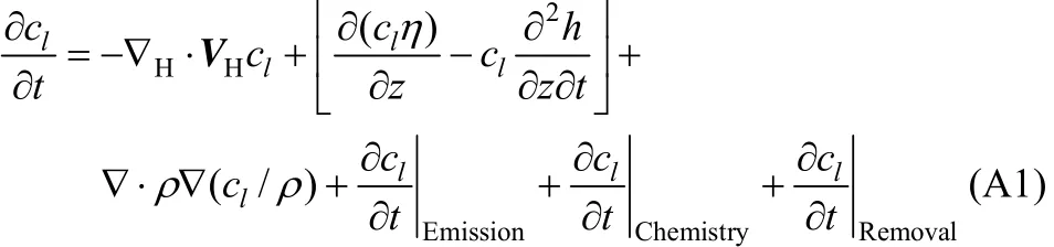
The governing equation of model CAMx is an Eulerian continuity equation that describes the time dependency of average species concentration within each grid cell volume as a sum of all physical and chemical processes operating in that volume. The equation is expressed in terrain-following height coordinates as follows:where clis the concentration of component l, VHis the horizontal wind vector, η is the net vertical transport rate, h is the layer interface height, ρ is atmospheric density, and K is the turbulent exchange coefficient. The continuity Eq. (A1) is replaced by an approach that calculates the separate contribution of each transport and diffusion process (emission, advection, diffusion, chemistry, and removal) to concentration change within each grid cell. These equations are as follows.
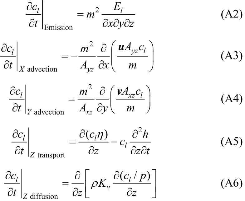
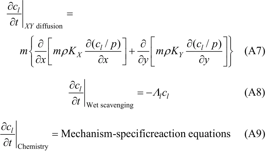
where Elis the local species emission rate, ciis species concentration (μmol·m−3for gasses, μg·m−3for aerosols), Eiis the local species emission rate (μmol·s−1for gasses, μg·s−1for aerosols), t is time step length (s), u and v are the east-west (χ) and north-south (y) horizontal wind components (m·s−1), respectively, Aχzand Ayzare cross-sectional areas of cells (m2) in the y-z and χ-z planes, m is the ratio of the transformed distance on various map projections to true distance, and Λlis the wet scavenging coefficient (s−1).
2013-08-15, accepted 2013-10-22.
* To whom correspondence should be addressed. E-mail: dcecbz@tsinghua.edu.cn
猜你喜欢
中学生学习报(2022年20期)2022-05-07
Chinese Physics B(2022年1期)2022-01-23
小天使·五年级语数英综合(2016年11期)2017-05-08
小天使·五年级语数英综合(2016年10期)2016-10-12
小天使·五年级语数英综合(2016年9期)2016-10-09
作文周刊·小学五年级版(2016年5期)2016-06-29
小天使·三年级语数英综合(2016年5期)2016-05-14
小天使·六年级语数英综合(2016年9期)2016-05-14
 Chinese Journal of Chemical Engineering2014年6期
- Chinese Journal of Chemical Engineering的其它文章
- Phase Behavior of Sodium Dodecyl Sulfate-n-Butanol-Kerosene-Water Microemulsion System*
- A LCA Based Biofuel Supply Chain Analysis Framework*
- Modeling and Optimization for Short-term Scheduling of Multipurpose Batch Plants*
- Symbiosis Analysis on Industrial Ecological System*
- Removal of Thiophenic Sulfur Compounds from Oil Using Chlorinated Polymers and Lewis Acid Mixture via Adsorption and Friedel-Crafts Alkylation Reaction*
- Unified Model of Purification Units in Hydrogen Networks*