
Diagnostic Study of Global Energy Cycle of the GRAPES Global Model in the Mixed Space-Time Domain
2014-12-14 06:58ZHAOBin赵滨andZHANGBo张博
关键词:张博
ZHAO Bin(赵滨)and ZHANG Bo(张博)
National Meteorological Center,Beijing 100081
Diagnostic Study of Global Energy Cycle of the GRAPES Global Model in the Mixed Space-Time Domain
ZHAO Bin(赵滨)and ZHANG Bo∗(张博)
National Meteorological Center,Beijing 100081
Some important diagnostic characteristics for a model’s physical background are reflected in the model’s energy transport,conversion,and cycle.Diagnosing the atmospheric energy cycle is a suitable way towards understanding and improving numerical models.In this study,formulations of the“Mixed Space-Time Domain”energy cycle are calculated and the roles of stationary and transient waves within the atmospheric energy cycle of the Global-Regional Assimilation and Prediction System(GRAPES)model are diagnosed and compared with the NCEP analysis data for July 2011.Contributions of the zonal-mean components of the energy cycle are investigated to explain the performance of numerical models.
Mixed Space-Time Domain energy cycle,energy reservoir,energy conversion,stationary wave, transient wave,GRAPES model
1.Introduction
Atmospheric systems such as cyclones and anticyclones are measured in terms of their kinetic energy (KE)(Storch et al.,2012),and those systems that are intensifying or weakening are often defined as gaining or losing KE(Luo,1994).Therefore,knowledge regarding the sources and sinks of KE in this context is very important(Li and Zhu,1995;Gao et al.,2006).
The total energy of the whole atmosphere will remain constant under adiabatic motion and the only source and sink of KE should be the available potential energy(APE).The APE can be considered as the difference between the total potential energy and minimum potential energy,and we can state that APE should vanish when the system’s distribution becomes universally horizontal and stable.However,the general motion of the atmosphere is not adiabatic;the presence of friction should alter KE directly,and conversion between APE and KE should be considered as the generation and dissipation energy within the whole life cycle of the atmospheric motions.
Supported by the National Nature Science Foundation of China(41305091)and China Meteorological Administration Special Fund for Numerical Prediction(GRAPES).
∗Corresponding author:zhaob@cma.gov.cn.
©The Chinese Meteorological Society and Springer-Verlag Berlin Heidelberg 2014
Lorenz(1955)developed a life cycle for energy conversions and defined a series of formulations to represent such conversions from APE to KE.He subdivided APE and KE into mean and eddy forms.The eddy form is the deviation from the mean form and the mean form can convert into the eddy form by eddytransport of sensible heat from low to high latitudes. In his energy cycle process,the general circulation can be characterized as a conversion of zonal APE,which is generated by low-latitude heating and high-latitude cooling,to eddy APE,then to eddy kinetic energy and to zonal mean KE.The conversion between the two forms of energy involves horizontal and vertical transport of momentum and sensible heat.The dissipation and generation terms within the life cycle can barely be estimated directly,and they are only a few balance terms in the budget equations.
This life cycle can be used to distinguish different contributions from different synoptic-scale and general circulation processes.It should give an intuitive judgment for evaluating the sources of different model performances.With regard to the Hadley cell,this largescale system involves a conversion from mean APE to mean KE(Dickinson,1969;Wu,1987),and for the barotropic atmosphere,the rate of transport between the eddy and mean KE is given by the product of the eddy transport if the momentum and gradient of mean angular rotation are both taken in the north-south direction.Concerning the baroclinic atmosphere(Stone, 1978),by the eddy transport of sensible heat from low to high latitudes,the mean APE converts into eddy APE and the eddy conversion from APE to KE is given by vertical motion and temperature within the latitudinal circle.Thus,it is a result of warm air rising and cold air sinking(Stein,1986;Huang and Vincent, 1998).In terms of the real atmosphere,the entire energy life cycle should display a complete conversion from APE to KE.
Oort(1964,1983)used the classical Lorenz energy cycle concept to estimate the reservoirs of APE and KE,together with related sources and sinks for the Northern Hemisphere.Steinheimer et al.(2008) estimated the conversion of Lorenz theory both in gridscale processes and subgridscale processes obtained from parameterization schemes.Their results showed that the subgridscale processes contributed significantly to the Lorenz energy cycle and the total dissipation terms of the subgridscale were more intense than what all earlier gridscale estimates had indicated.
Lorenz formulas can be introduced in the space domain,and we can further acquire the energy value in the mixed space and time domain,the so-called“Mixed Space-Time Domain”energy cycle.The eddy energy is subdivided into stationary and transient waves.The stationary form is the time mean and a result of diabatic and orographic forcing.The transient form is the departure from the time mean and a result of baroclinic instability of zonal mean flow(Simmons and Hoskins,1978,1980).
Ulbrich and Speth(1991)expanded the Lorenz classical process to give a series of detailed formulations for the“Mixed Space-Time Domain”energy cycle(Arpe et al.,1986),and examined the role of stationary and transient waves within the atmospheric energy cycle with the ECMWF data for winter and summer.Their results showed that all terms of the energy cycle related to stationary waves reveal a predominance of the planetary scale while the transient waves are governed by synoptic-scale waves.
In the present study,an approach based on the“Mixed Space-Time Domain”energy cycle is adopted.The formulations of the energy cycle are calculated,and the role of stationary and transient waves within the atmospheric energy cycle from the Global-Regional Assimilation and Prediction System (GRAPES)is firstly diagnosed and compared with NCEP Final Operational Global Analysis(FNL)data for July 2011.Three main kinds of considerable processes(planetary scale,barotropic conversion,and baroclinic conversion)are examined separately in order to investigate in detail the characteristics and features of energy cycle and its component contribution. The zonal-mean components of the energy cycle are investigated to diagnose the performance of numerical integrations.The forecast results at different lead times are used to explain the reason for deteriorating forecast performance.
2.Method
By following Ulbrich and Speth(1991)’s energy cycle framework(illustrated in Fig.1),all the energy reservoirs and conversions are calculated in this study with Ulbrich and Speth’s detailed formulations. Zonal available potential energy(AZ)and zonal kinetic energy(KZ)are zonal APE and KE.Stationary eddy available potential energy(ASE)and transient eddy available potential energy(ATE)are stationary and transient eddy APE,and the stationary and transient eddy KE is named KSE and KTE,respectively. Besides energy reservoirs,some terms of the energy cycle,such as CZ(conversion from AZ to KZ),CAS (conversion from AZ to ASE),CAT(conversion from AZ to ATE),CES(conversion from ASE to KSE), CET(conversion from ATE to KTE),CKS(conversion from KZ to KSE),CKT(conversion from KZ to KTE),and the nonlinear conversions between stationary and transient terms(CATE and CKTE)all play important roles in the global energy cycle process and can be regarded as an important benchmark to estimate the basic model performance.
3.Data

Fig.1.Diagram of the global atmospheric energy cycle in the Mixed Space-Time Domain.Arrows indicate orientation of conversions corresponding to the definitions of parameters(from Ulbrich and Speth,1991).Note:G denotes generation of potential energy;D denotes dissipation of kinetic energy.
The GRAPES model daily forecast data for July 2011 with four different lead times of 24,72,120,and 168 h are used.The model resolution is selected as 0.5°and it is initialized with global 1200 UTC analyses of the NCEP FNL data.Archived GRAPES model data consist of geopotential height,temperature,specific humidity,zonal and meridional wind,and vertical wind for 29 pressure levels(1000,962.5,925,887.5, 850,800,750,700,650,600,550,500,450,400,350, 300,275,250,225,200,175,150,125,100,70,50, 30,20,and 10 hPa).NCEP FNL data are selected as the analysis data for comparison and are interpolated from 1.0°to 0.5°grid,and vertically from 26 to 29 pressure levels.NCEP global forecast(not analysis)data are also selected for the same time period and the same horizontal and vertical resolutions for comparison.
4.Results
4.1 The global energy cycle for July 2011
As a preliminary work for the energy cycle analysis,it is necessary to evaluate the performance of the GRAPES model and provide an intuitive impression of the quality of the FNL data,which serve as the comparative observation.In the classical treatment of statistical verification for different model forecasts, root-mean-square-error(RMSE)is a predominant index used as a measure of model forecast performance. Temperature and wind velocity are the main variables involved in the calculation of energy cycle and conversion terms.Figure 2 depicts the global averaged RMSE for temperature and wind velocity against the FNL analysis data and NCEP BUFR(Binary Universal Form of the Representation of meteorological data) sounding data.The latter dataset is chosen as the observation,which is only distributed between 850 and 50 hPa.Figure 2a shows that the maxima of temperature RMSE are mostly concentrated within 200 hPa,and with increasing lead time,RMSE grows from 1.59 K(24 h)to 3.80 K(168 h).Meanwhile,in Fig. 2c,the maxima of wind velocity RMSE are located within 250 hPa,and with increasing lead time,RMSE rises from 6.14 m s-1(24 h)to 16.16 m s-1(168 h). The RMSEs of GRAPES model outputs relative to the FNL data in Fig.2b and 2d present a similar pattern to that in Figs.2a and 2c.Temperature RMSE at different lead times in Fig.2c is consistently smaller
than that in Fig.2a(e.g.,at 200 hPa,1.09 K for 24 h and 3.53 K for 168 h).Moreover,wind velocity RMSE is smaller in Fig.2d than in Fig.2b at 120-h lead time and increases to 17.00 m s-1(168 h)at 250 hPa.This is possibly due to the GRAPES model being initiated with the FNL data.With respect to upper levels(above 50 hPa),where there are no comparative observations,large temperature and wind velocity RMSE maxima are observed to intensify with lead time.This will lead to strengthening potential energy and KE.
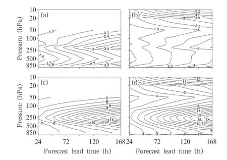
Fig.2.Global averaged RMSE for GRAPES produced (a,b)temperature(K)against(a,c)NCEP BUFR observation and(b,d)FNL analysis in July with different lead times.
Following Ulbrich and Speth’s work(1991),we have calculated the globally averaged energy cycle of the GRAPES model with different lead times and the results are shown in Fig.3.It is confirmed that the GRAPES model has the capability to reproduce the main features of the global energy cycle as compared with NCEP analysis data.AZ is converted into ASE and ATE;the stationary waves cannot be neglected compared with the transient ones,and ASE and ATE have about the same value.The nonlinear conversion between the two eddy available potential energy terms, i.e.,CATE,plays an important role in the global energy cycle and is directed from the stationary to the
transient reservoir of APE.It can be deduced that the damping of stationary temperature by horizontal transient fluxes of sensible heat is an important process in the global general circulation.
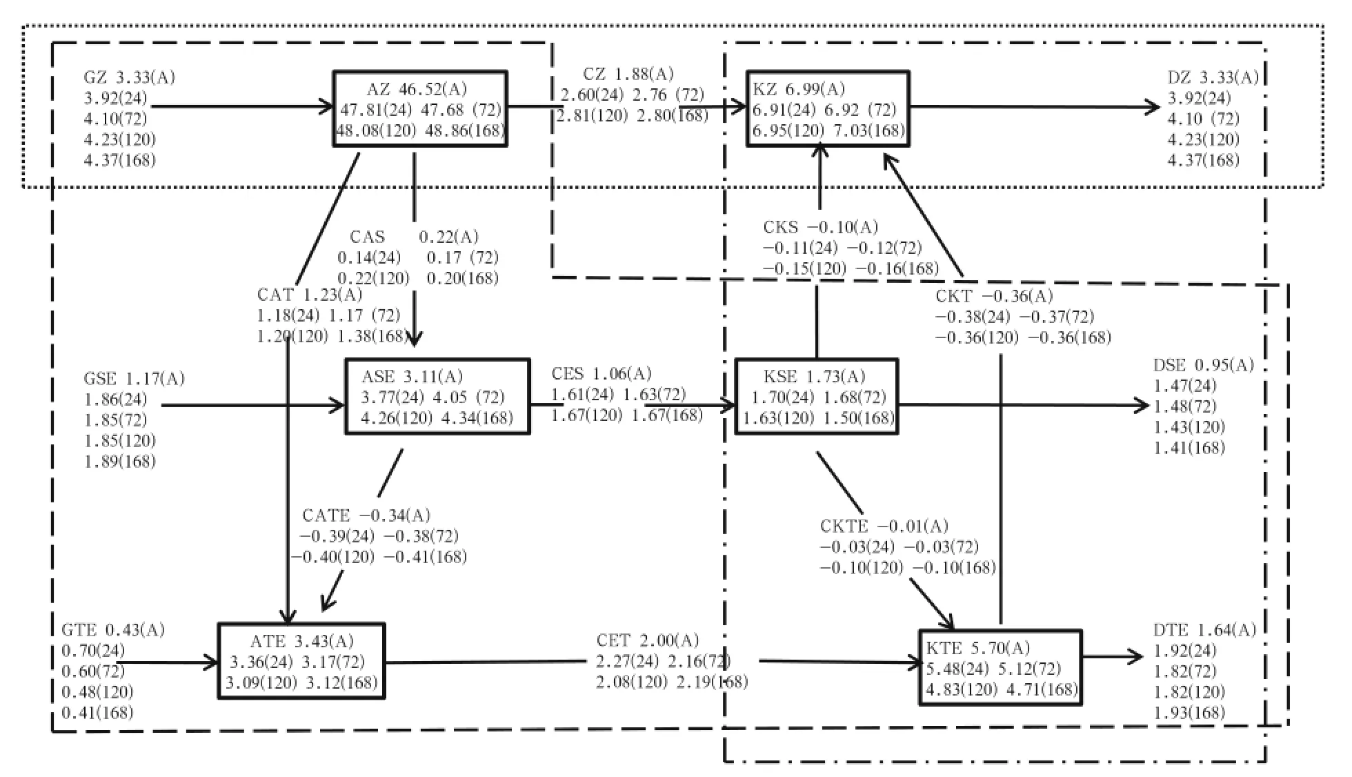
Fig.3.The global atmospheric energy cycle of GRAPES in July 2011.Various energy components(in boxes)are in J m-2,while conversions between the components are in W m-2.Numbers at the top indicate values based on NCEP FNL data,and 24,72,120,and 168 h are the different lead times from 1 to 7 days.The dotted frame refers to the planetary-scale(Hadley cell)process,the dashed frame refers to the barotropic process,and the dot-dashed frame refers to the baroclinic process.
With increased forecast lead time,AZ becomes larger,which reflects the meridional temperature gradient between high and low latitudes becoming steeper. This enhances zonal baroclinic processes, which increases the meridional heat flux and enhances the conversion from AZ to eddy potential energy,especially the conversion of the transient term,CAT.The stationary conversion of APE,i.e.,CAS,is just 1/6 of the magnitude of the transient conversion of CAT.
The zonal KE(i.e.,KZ)has a similar value to the sum of stationary and transient eddy KE(KSE and KTE),and the transient term is three times larger than the stationary term,while there is almost no global net conversion between the two eddy KE terms. Barotropic stationary and transient conversions(CKS and CKT)are directed from eddy KE to zonal KE. The zonal planetary-scale conversion CZ(from AZ to KZ)is about 1.5 times larger in GRAPES than in the NCEP analysis.
4.2 Planetary-scale processes
The globally averaged energy values are presented in Fig.3,which gives us an intuitive impression of how the global energy cycle works.It is also a useful diagnosis tool to analyze the source of the bias between different model forecasts.However,globally averaged values can barely depict the contributions and interrelations of special energy terms.More needs to be done to reveal detailed features.We further separate the framework of the energy cycle into three major processes:planetary-scale,barotropic,and baroclinic atmospheric processes.
With regard to planetary-scale processes,largescale systems such as the Hadley cell provide a conversion from zonal APE(AZ)to zonal KE(KZ).The AZ and KZ increase with the increasing lead time.Figure 4 shows the zonal mean temperature distribution of NCEP FNL analysis and the bias of the GRAPES forecast relative to FNL data at different lead times.As expected,the maximum overestimation is located at low levels near the equator and at high levels near the poles,and the overestimation becomes stronger with increasing lead time.This indicates that the strong warm bias in the low latitudes increases the meridional temperature gradient,which leads to stronger AZ.Concerning the CZ term,which represents the conversion between AZ and KZ,this reflects the zonal features of the vertical wind and temperature.When warm air rises and cold air sinks,CZ>0 and shows Hadley cell features.In contrast,when CZ<0,it shows the features of the Ferrel cell.In Fig.3,it presents positive values of CZ,so it reflects a Hadley cell feature in planetary-scale processes.
4.3 Barotropic conversion
In this section,the barotropic conversion and KE are diagnosed.As discussed in Section 4.1,zonal KE (KZ)is the sum of the stationary and transient eddy KE,while KSE is about 1/3 of KTE and there is almost no net global conversion between the two eddy terms.The zonal distribution of KTE(Fig.5)shows that the maxima in the Southern Hemisphere are displaced northward at the location of the zonal mean jet (50°S)and the maxima in the Northern Hemisphere
are displaced southward in the opposite latitudes. With increasing lead time,the strong western flow decreases in the upper troposphere(near 300 hPa)and stratosphere(near the top of the model),which leads to a decreasing of the global averaged energy value.

Fig.4.(a)Zonal averaged temperature distribution of FNL and(b)-(e)biases of GRAPES relative to FNL with different lead times(1-7 days,i.e.,D+1 to D+7).

Fig.5.Transient eddy kinetic energy(KTE)in July(J m-2Pa-1).(a)FNL data,and(b)24-,(c)72-,(d)120-, and(e)168-h GRAPES forecast.
The stationary eddy KE(KSE)displays a very different pattern to the transient one(Fig.6).The comparatively weak maxima are presented at the locations of 30°S,15°N,and 45°N,separately,and are associated with the zonal mean jets in both hemispheres. Another maximum appears in high latitudes of the Southern Hemisphere,which is related to the polar jet.With increasing leading time,the four weaker maxima decrease significantly.A band of high energy values presents in the Southern Hemisphere over 100 hPa due to the presence of a large zonal wind jet at the upper 30-hPa level,which causes a strengthening of KSE.
As mentioned before,the nonlinear conversion be tween KSE and KTE is directed from KSE to KTE, and it is difficult to determine the symbol of the global averaged value because it is approximately zero.However,the zonal mean distribution of transient eddy momentum against or along the direction of the stationary eddy momentum gradient can be explained. The zonal mean distribution of the nonlinear conversion CKTE shows a pair of strong maxima in Fig.7. Comparing the location with respect to the zonal mean
contribution of KSE and KTE,we find that the maximum of the nonlinear conversion is displaced near the location of the maximum KTE and minimum KSE. This means that the strong nonlinear conversion can be considered as a physical mechanism forcing the atmosphere to a more uniform state.Figure 7 shows that as the lead time increases,the maximum nonlinear conversion value becomes weaker,which indicates a weakening of the local contribution.

Fig.6.As in Fig.5,but for the stationary eddy kinetic energy(KSE)in July(J m-2Pa-1).

Fig.7.Distributions of the conversion term CKTE(from KTE to KSE;10-6W m-2Pa-1)in July.(a)FNL data, and(b)24-,(c)72-,(d)120-,and(e)168-h GRAPES forecast.
CKTE is a very important nonlinear conversion term and its positive or negative value indicates the direction of transfer between transient waves and stationary waves.Moreover,the strength of KSE can be used as a basis to determine the jet intensity changes.When CKTE is positive,heat transport is transferred from transient waves to stationary waves, which strengths KSE.Conversely,if CKTE is negative,heat transport is directed into transient waves, resulting in a weakening of KSE.The result obtained by Ulbrich and Speth(1991)showed that a strengthening of KSE corresponded to local jet maxima while a weakening prevailed over the jet entrance regions.
Figure 7 shows the conversion term CKTE from FNL analysis and GRAPES forecast,while the CKTE in the Southern Hemisphere is depicted in Fig.8. It is seen that in the FNL analysis,positive values are mainly found downstream of the jet maxima over Southwest Pacific,while negative values are distributed in the jet entrance regions over Southeast Atlantic where wind velocity is relatively weak.The distribution of positive and negative local values and jet regions verifies Ulbrich’s conclusion.Compared with the FNL analysis,the strength of the local jet in the GRAPES forecast becomes gradually weaker with increased lead time,while the corresponding CKTE decreases significantly,together leading to the dissipation of KSE.Until 7 days,the positive values over the local jet maxima show a clear decreasing trend,while the corresponding jet is significantly weaker than in the FNL analysis.It can be concluded that CKTE can be used to determine stationary wave changes,and act as an indicator of the jet intensity features.
4.4 Baroclinic conversion
For the baroclinic conversion process,the global averaged values reported in Fig.3 indicate how this process is working.With increased lead time,the conversion from zonal APE to stationary eddy APE remains constant.As a result of the meridional temperature gradient increasing,meridional transport of sensible heat enhances,which causes an increase in the conversion CAT,transferring energy from zonal to transient eddy APE.
In order to compare details of the process associated with baroclinic conversion,the zonal contributions of ASE and ATE are plotted in Fig.9.Larger ASE values appear in both the Southern and Northern Hemispheres.In the Northern Hemisphere,the largest ASE is found below 850 hPa between 20°and 60°N,and the second largest ASE is seen between 400 and 200 hPa around 30°N.However,in the Southern Hemisphere,the largest ASE occurs between 850 and 700 hPa and further south of 60°S,with the maximum value greater than 30 J m-2Pa-1.In contrast to ASE,the zonal mean distribution of ATE has a similar structure to KTE(Fig.5).The maximum value of transient eddy potential energy ATE is only about half that of ASE.With increased lead time,the maximum value of ASE increases and ATE decreases slightly.
In terms of the zonal mean distribution of ASE, Fig.10 shows that the maxima of ASE are associated with the linear conversion term CAS.The zonal contribution of stationary conversion is negative over 200-400 hPa at 30°N,corresponding to similar conversion rates of ASE maximizing at a similar location. The same coincidence can be seen in high latitudes of the Southern Hemisphere.The zonal mean contribution to the conversion from zonal to transient eddy APE,i.e.,CAT,is determined by the meridional temperature gradient.Comparing CAT(Fig.10)with ATE(Fig.9)reveals that a coincidence in the maximum energy value with conversion terms is apparent.The conversion value increases over low levels in the Southern Hemisphere with increasing lead time. This is determined by the decreasing of vertical stability and,simultaneously,the decreasing of transient sensible heat transport.The coincidence in the distribution of CAS is found to be very similar to that observed for the transient term with respect to midtropospheric values.This indicates that the baroclinic
process associated with the stationary wave is comparable to that associated with the transient wave.
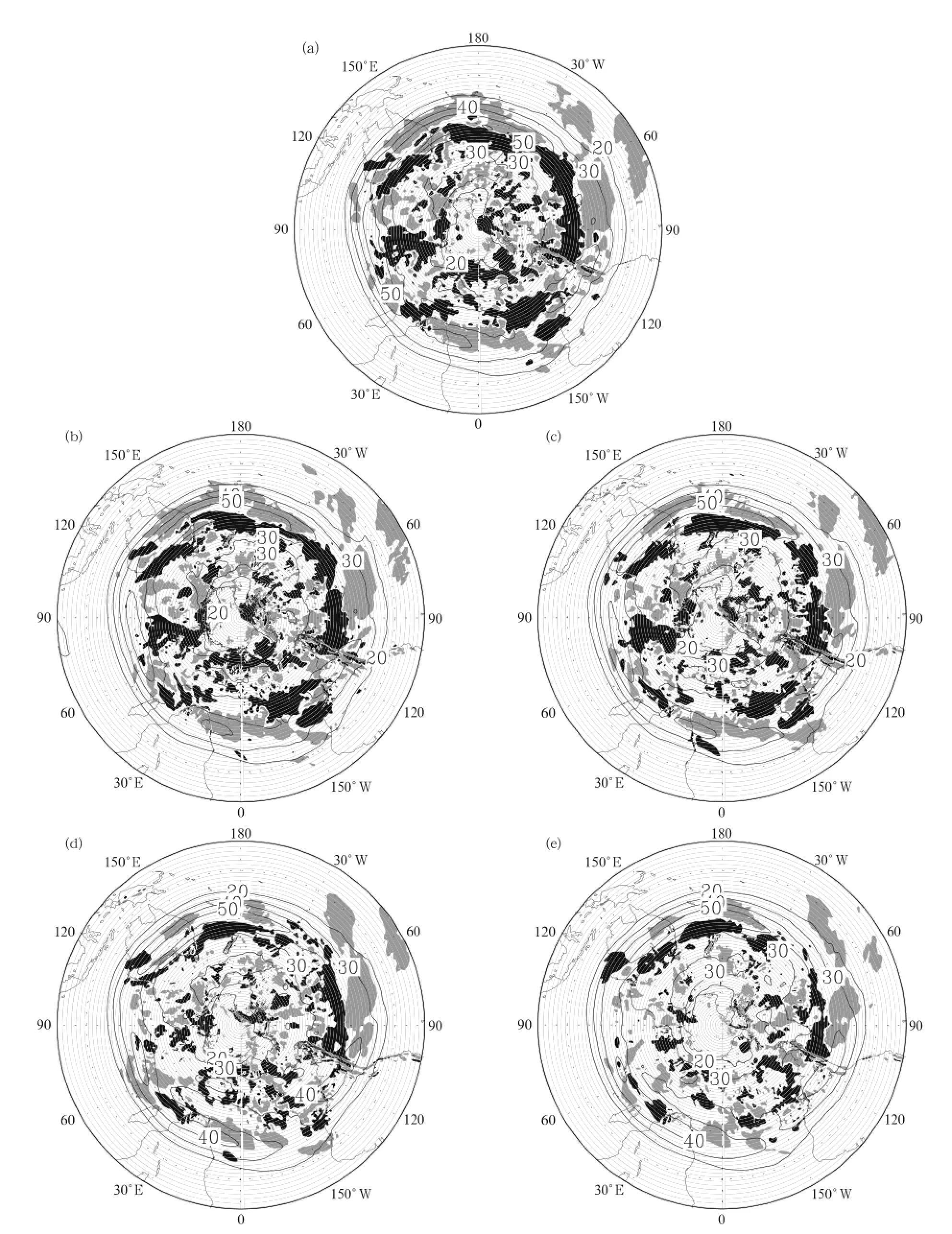
Fig.8.Wind velocity(m s-1)at 250 hPa in July 2011 in the Southern Hemisphere.Shaded areas depict the local contributions to CKTE greater than 50×10-6W m-2Pa-1(dark)and lower than-50×10-6W m-2Pa-1(light).(a) FNL data,and(b)24-,(c)72-,(d)120-,and(e)168-h GRAPES forecast.

Fig.9.(a1-e1)Stationary eddy available potential energy(ASE)and(a2-e2)transient eddy available energy(ATE)(J m-2Pa-1)in July.(a1-a2)FNL data,and(b1-b2)24-,(c1-c2)72-,(d1-d2)120-,and(e1-e2)168-h forecast.

Fig.10.As in Fig.9,but for the conversion terms CAS(a1-e1)and CAT(a2-e2)(10-6W m-2Pa-1)in July.
The nonlinear conversion CATE is directed from ASE to ATE.Local zonal mean values of this nonlinear conversion are depicted in Fig.11.The maximum contribution to the global averaged energy is located at lower levels over Antarctica,where the maximum value of ASE presents.It is considered that this kind of energy conversion does not originate from the zonal reservoir of AZ,but from the stationary eddy APE’s nonlinear interactions.The maximum ASE above the troposphere at 30°N is not associated with the strong nonlinear conversions.The negative values of CATE is seen to intensify over Antarctica with increased
lead time. The nonlinear conversion is thought as the horizontal heat transport by transient waves(Lau, 1982)and a negative value means that the heat transport is directly from warm to cold regions.

Fig.11.As in Fig.7,but for CATE(ATE to ASE;10-6W m-2Pa-1)in July.
As the maximum zonal mean CATE appears at 700 hPa in the Southern Hemisphere,we choose to analyze the nonlinear conversion CATE at 700-hPa in the Southern Hemisphere(Fig.12).With regard to the FNL analysis,some negative and positive values of CATE are located around Antarctica,coinciding with regions of relatively warm and cold air.We superimpose temperature on CATE,and see that the distribution coincides with the horizontal heat transport by the transient waves.When heat is transported against the local temperature gradient by transient waves,meaning that heat transport is directed into the warm region,the CATE value is positive.In contrast,a negative value indicates that the heat transport is directed into the cold region.Compared with FNL data,the GRAPES forecast data show a larger temperature gradient and increasing negative values.
4.5 Comparison with NCEP-GFS
According to the aforementioned analysis of the atmospheric energy cycle,the main characteristics of the energy cycle is now used to aid in traditional verification of model performance.Real forecast data with the same resolution as that of FNL data from the NCEP Global Forecast Systems(NCEP-GFS)are used to compare the features of the energy cycle with the GRAPES model.The same 31 days of analysis are carried out and monthly averages are considered.
Firstly,the anomaly correlation coefficient(ACC) is calculated for geopotential height at 500 hPa. We use wavelet analysis and our verification procedure include a separation of the waves with different zonal wave numbers.The long waves of the planetary scale(zonal wavenumbers 0-3),synoptic scale waves(zonal wavenumbers 4-9),and small-scale waves (zonal wavenumbers 10-20)are distinguished separately.We assume that fast moving waves are synoptic or small scale,and slowly moving ones are predominantly planetary scale(Kung,1988).
In Fig. 13,the separation into the different wavenumber groups is shown in order to compare the performance of NCEP forecast and GRAPES forecast. With respect to NCEP forecast results,the ACC of GRAPES falls behind with different lead times.The bias at 168 h is approximately 0.03 and all verification indices are significant at the 95%confidence level. The planetary-scale contribution is roughly similar to the aggregate performance. However,the synoptic scale and shorter scale represent some differences:for the synoptic scale(wavenumbers 4-9),the confidence interval becomes larger at 168 h,meaning that the standard deviation of ACC bias also becomes larger. Therefore,the bias can barely satisfy the 95%confidence level.For the shorter scale(wavenumbers 10-20),the bias of model performance becomes more statistically insignificant after 48 h.We conclude that significant bias is reflected on the large and meso scales, and is roughly equal on the smaller scale.

Fig.12.Temperature(K)at 700 hPa in July 2011 in the Southern Hemisphere.Shaded areas depict local contributions to CATE greater than 50×10-6W m-2Pa-1(dark)and lower than-50×10-6W m-2Pa-1(light).(a)FNL data,and (b)24-,(c)72-,(d)120-,and(e)168-h forecast.

Fig.13.Monthly mean of 500-hPa geopotential height ACC for GRAPES and NCEP-GFS with different lead times of 1-7 days.(a)Total statistical score,(b)planetary scale(wavenumbers 0-3),(c)synoptic scale(wavenumbers 4-9), and(d)short scale(wavenumbers 10-20).Note:“w.r.t.”means“with regard to.”
Figure 14 shows the energy values for the global integrals of NCEP-GFS with different lead times.In contrast to the GRAPES model,it is generally accepted that most energy values calculated by baroclinic and barotropic processes are roughly similar in July.The primary difference lies in the conversion of zonal APE to zonal KE,which is a result of the planetary-scale processes.AZ of NCEP-GFS is larger than in GRAPES,which means that NCEP-GFS has a steeper meridional temperature gradient between the high and low latitudes.The conversion term CZ of NCEP-GFS is smaller than in GRAPES,which is mainly due to the simulated weak vertical wind.Due to the hydrostatic assumption,NCEP-GFS simulates weaker vertical air motion than GRAPES,leading to the nonlinear conversion CZ becoming smaller.All of these features will seriously affect the Hadley cell simulation.KZ of GRAPES is larger than that of NCEP-GFS,mainly because of the zonal mean wind amplitude being too large.It should be noted at this point that the difference in model performance between GRAPES and NCEP-GFS is mainly reflected in the large-scale process,and such a conclusion is consistent with the results obtained via traditional verification in Fig.13.Furthermore,detailed characteristics should be investigated and compared with a full analysis of unique energy cycle processes.

Fig.14.The global atmospheric energy cycle in the Mixed Space-Time Domain for NCEP-GFS in July 2011.Various energy components(in boxes)are in J m-2,while conversions between the components are in W m-2.Numbers at the top indicate values based on NCEP FNL data,and 24,72,120,and 168 h are the different lead times from 1 to 7 days. The dashed box indicates the large difference of NCEP-GPS with the GRAPES model.
5.Summary
An investigation on the atmospheric energy cycle was carried out by using GRAPES forecast data,with a focus on the role of model performance at different lead times.Three main atmospheric-scale processes were diagnosed separately and the characteristics of stationary and transient eddy energy terms and their conversions were calculated and presented.The results show that:
(1)The GRAPES model has the capability to reproduce the main characteristics of the global energy cycle as compared with NCEP FNL analysis data.
(2)ASE and ATE have approximately the same values and the nonlinear conversion is directed from the stationary to the transient.
(3)Barotropic conversions(CKS and CKT)are directed from eddy kinetic energy to zonal kinetic energy,and the kinetic energy of stationary eddy is about 1/3 of that of the transient eddy.
(4)With increasing forecast lead time,AZ becomes larger and the zonal conversion CZ(from AZ to KZ)in GRAPES is around 1.5 times larger than in the NCEP analysis.
(5)In contrast with traditional verification,the energy cycle diagnosis can help to derive statistical scores and identify the source of model differences.
This study on the diagnosis of the energy cycle is at a preliminary stage in terms of operational application.There are some areas of work that need to be improved and some problems that should be noted. For example,only short-term integrations of forecast data were collected for analysis in order to acquire stable performances of energy values.Low-resolution and long-term integrations should be run for“seasonal forecasts.”Moreover,we have recognized that diagnosis of the energy cycle can be achieved with a similar conclusion to traditional verification methods,but how to combine traditional verification methods with this energy cycle diagnosis for model evaluation remains to be examined.These problems should be discussed in future investigations.
Arpe,K.,C.Brancovic,E.Oriol,et al.,1986:Variability in time and space of energetics from a long series of atmospheric data produced by ECMWF.Beitr. Phys.Atmos.,59,321-355.
Dickinson,R.E.,1969:Theory of planetary wave-zonal flow interaction.J.Atmos.Sci.,26,73-81.
Gao Hui,Chen Longxun,He Jinhai,et al.,2006:Characteristics of zonal propagation of atmospheric kinetic energy at equatorial region in Asia.Acta Meteor. Sinica,20,86-94.
Huang,H.-J.,and D.G.Vincent,1988:Daily spectral energy conversions of the global circulation during 10-27 January 1979.Tellus,40A,37M9.
Kung,E.C.,1988:Spectral energetics of the general circulation and time spectra of transient waves during the FGGE year.J.Climate,1,5-19.
Lau,N.C.,and A.H.Oort,1982:A comparative study of observed Northern Hemisphere circulation statistics based on GFDL and NMC analyses.Part II: Transient eddy statistics and the energy cycle.Mon. Wea.Rev.,110,889-906.
Li Qingquan and Zhu Qiangen,1995:Analysis on the source and sink of kinetic energy of atmospheric 30-60-day period oscillation and the probable causes. Acta Meteor.Sinica,9,420-431.
Lorenz,E.N.,1955:Available potential energy and the maintenance of the general circulation.Tellus,7, 157-167.
Luo Zhexian,1994:Effect of energy dispersion on the structure and motion of tropical cyclone.Acta Meteor.Sinica,8,51-59.
Oort,A.H.,1964:On estimates of the atmospheric energy cycle.Mon.Wea.Rev.,92,483-493.
—-,1983:Global Atmospheric Circulation Statistics 1958-1973,Volume 14,NOAA Professional Paper. U.S.Department of Commerce/NOAA,180.
Simmons,A.J.,and B.J.Hoskins,1978:The life cycles of some nonlinear baroclinic waves.J.Atmos.Sci., 35,414-432.
—-,and—-,1980:Barotropic influences on the growth and decay of nonlinear baroclinic waves.J.Atmos. Sci.,37,1679-1684.
Stein, C., 1986: Das zeitliche Zusammenwirken baroklinerEnergieumwandlungen durch grogrfiumige Wellen in derAtmosph/ire. Diplomarbeit, Institut fiir Geophysik und Meteorologie der Universit/it zu K61n.
Steinheimer,M.,M.Hantel,and P.Bechtold,2008:Convection in Lorenz’s global energy cycle with the ECMWF model.Tellus,60A,1001-1022.
Stone,P.H.,1978:Baroclinic adjustment.J.Atmos. Sci.,35,561-571.
Storch,J.S.,C.Eden,and I.Fast,2012:An estimate of the Lorenz energy cycle for the world ocean based on the STORM/NCEP simulation.J.Phys.Oceanogr., 42,2185-2205.
Ulbrich,U.,and P.Speth,1991:The global energy cycle of stationary and transient atmospheric waves: Results from ECMWF analyses.Meteor.Atmos. Phys.,45,125-138.
Wu Rongsheng,1987: Energy,energy flux and Lagrangian of Rossby wave. Acta Meteor. Sinica, 1,143-150.
:Zhao Bin and Zhang Bo,2014:Diagnostic study of global energy cycle of the GRAPES global model in the mixed space-time domain.J.Meteor.Res.,28(4),592-606,
10.1007/s13351-014-3072-0.
(Received October 16,2013;in final form June 17,2014)
The results show that the GRAPES model has the capability to reproduce the main features of the global energy cycle as compared with the NCEP analysis.Zonal available potential energy(AZ)is converted into stationary eddy available potential energy(ASE)and transient eddy available potential energy(ATE),and ASE and ATE have similar values.The nonlinear conversion between the two eddy energy terms is directed from the stationary to the transient.AZ becomes larger with increased forecast lead time,reflecting an enhancement of the meridional temperature gradient,which strengthens the zonal baroclinic processes and makes the conversion from AZ to eddy potential energy larger,especially for CAT(conversion from AZ to ATE).The zonal kinetic energy(KZ)has a similar value to the sum of the stationary and transient eddy kinetic energy.Barotropic conversions are directed from eddy to zonal kinetic energy.The zonal conversion from AZ to KZ in GRAPES is around 1.5 times larger than in the NCEP analysis.The contributions of zonal energy cycle components show that transient eddy kinetic energy(KTE)is associated with the Southern Hemisphere subtropical jet and the conversion from KZ to KTE reduces in the upper tropopause near 30°S.The nonlinear barotropic conversion between stationary and transient kinetic energy terms(CKTE) is reduced predominantly by the weaker KTE.
猜你喜欢
锦州医科大学报(2022年2期)2022-05-07
师道·教研(2021年8期)2021-09-22
Chinese Physics B(2021年5期)2021-05-24
造纸信息(2019年7期)2019-09-10
消费电子(2017年5期)2017-05-25
消费电子(2017年5期)2017-05-25
微型小说选刊(2016年20期)2017-01-19
福建中学数学(2016年8期)2016-12-03
创业邦(2016年3期)2016-03-17
遗传(2015年10期)2015-01-03
 Journal of Meteorological Research2014年4期
- Journal of Meteorological Research的其它文章
- Chinese Contribution to CMIP5:An Overview of Five Chinese Models’Performances
- Track of Super Typhoon Haiyan Predicted by a Typhoon Model for the South China Sea
- Variations in Regional Mean Daily Precipitation Extremes and Related Circulation Anomalies over Central China During Boreal Summer
- The Persistent Heavy Rainfall over Southern China in June 2010: Evolution of Synoptic Systems and the Effects of the Tibetan Plateau Heating
- Overview of the Major 2012-2013 Northern Hemisphere Stratospheric Sudden Warming:Evolution and Its Association with Surface Weather
- Characteristics of Meteorological Factors over Different Landscape Types During Dust Storm Events in Cele,Xinjiang,China