
Flux Footprint Climatology Estimated by Three Analytical Models over a Subtropical Coniferous Plantation in Southeast China
2015-01-05 02:02ZHANGHui张慧andWENXuefa温学发
关键词:张慧
ZHANG Hui(张慧)and WEN Xuefa(温学发)
1 Jinzhou Ecology and Agriculture Meteorological Center,Jinzhou 121001
2 Key Laboratory of Ecosystem Network Observation and Modeling,Institute of Geographic Sciences and Natural Resources Research,Chinese Academy of Sciences,Beijing 100101
Flux Footprint Climatology Estimated by Three Analytical Models over a Subtropical Coniferous Plantation in Southeast China
ZHANG Hui1(张慧)and WEN Xuefa2∗(温学发)
1 Jinzhou Ecology and Agriculture Meteorological Center,Jinzhou 121001
2 Key Laboratory of Ecosystem Network Observation and Modeling,Institute of Geographic Sciences and Natural Resources Research,Chinese Academy of Sciences,Beijing 100101
Spatial heterogeneity poses a major challenge for the appropriate interpretation of eddy covariance data. The quantification offootprint climatology is fundamentalto improving our understanding ofcarbon budgets, assessing the quality of eddy covariance data,and upscaling the representativeness of a tower flux to regional or global scales.In this study,we elucidated the seasonal variation of flux footprint climatologies and the major factors that influence them using the analytical FSAM(Flux Source Area Model),KM(Kormann and Meixner,2001),and H(Hsieh et al.,2000)models based on eddy covariance measurements at two and three times the canopy height at the Qianyanzhou site of ChinaFLUX in 2003.The differences in footprints among the three models resulted from different underlying theories used to construct the models. A comparison demonstrated that atmospheric stability was the main factor leading to differences among the three models.In neutral and stable conditions,the KM and FSAM values agreed with each other,but they were both lower than the H values.In unstable conditions,the agreement among the three models for rough surfaces was better than that for smooth surfaces,and the models showed greater agreement for a low measurement height than for a high measurement height.The seasonal flux footprint climatologies were asymmetrically distributed around the tower and corresponded well to the prevailing wind direction, which was north-northwest in winter and south-southeast in summer.The average sizes of the 90%flux footprint climatologies were 0.36-0.74 and 1.5-3.2 km2at altitudes of two and three times the canopy height,respectively.The average sizes were ranked by season as follows:spring>summer>winter>autumn.The footprint climatology depended more on atmospheric stability on daily scale than on seasonal scale,and it increased with the increasing standard deviation of the lateral wind fluctuations.
eddy covariance,flux footprint,flux footprint climatology,model comparison
1.Introduction
Spatial heterogeneity poses a major challenge for the appropriate interpretation ofeddy covariance(EC) data(Baldocchi,2008;Kljun,2010a;Biermann et al., 2011;Leclerc et al.,2014).Flux footprint climatology is a practical method to illustrate the portion of the sampled landscape that contributes the most to EC vertical turbulent flux at a given point over long-term periods(Amiro,1998;Kljun,2010a;Cai et al.,2011; Aubinet et al.,2012;Zhang et al.,2012).This method is used to understand carbon budgets,assess the quality of EC data,and upscale the representativeness of a tower flux to regional or global scales(Rebmann et al.,2005;G¨ockede et al.,2008;Chen et al.,2012).
Flux footprint climatology,which is the long-term pattern of the flux footprint(Chen et al.,2009),provides a quantitative estimate of changes in the spatial representativeness of EC over time(Allen et al.,2011; Chen et al.,2011,2012).It is important to studywhether the factors affecting flux footprint climatology are the same as those affecting the flux footprint itself, such as wind direction,atmospheric stability,surface roughness length,and measurement height(Aubinet et al.,2012).It is not clear whether atmospheric stability,a parameter that fluctuates daily,strongly affects flux footprint climatology on monthly or seasonal scales.In addition,quantitative analysis to determine how much the size of the flux footprint climatology increases with measurement height is also necessary.Because trees grow taller over time,EC measurements are performed progressively closer to the canopy,which can impact the footprint climatology of flux measurements.
Analytical models are often used for estimating flux footprints due to their ease of coding compared with the Lagrangian stochastic models(Leclerc and Thurtell,1990;Kljun,2010b),large eddy simulations(Cai et al.,2010),and closure models(Sogachev and Lloyd,2004).Currently,analyticalmodels such as the FSAM(Flux Source Area Model)developed by Schmid(1994),the KM model by Kormann and Meixner(2001),and the H model by Hsieh et al. (2000),are widely adopted.However,the strength, weakness,and applicability of each model have not been fully demonstrated.How the three models differ with variations in measurement height,surface roughness length,and atmospheric stability needs to be assessed.
The objective of this study is to elucidate the seasonal variation of flux footprint climatologies and the major factors that influence them by using the analytical FSAM,KM,and H models based on eddy covariance measurements at two and three times the canopy height at the Qianyanzhou site of ChinaFLUX.ChinaFLUX is an observation and research network that uses eddy covariance and chamber methods to measure the exchanges of carbon dioxide,water vapor, and energy between the terrestrial ecosystem and the atmosphere in China(Yu et al.,2006).A comparison of the three models will be performed to evaluate their differences with changes in measurement height, surface roughness length,and atmospheric stability. Then,the three analytical footprint models are used to reveal the seasonal variations of the flux footprint climatologies.Finally,the major factors influencing the sizes of the flux footprint climatologies over the Qianyanzhou site are investigated.
The paper is organized as follows.Materials and methods are described in Section 2.Comparison of the three flux footprint models and the simulated seasonal variations of the flux footprint climatologies are presented in Section 3.Effects of atmospheric stability,wind fluctuations,and measurement height on the flux footprint climatology are discussed in Section 4. A summary and conclusions are given in Section 5.
2.Materials and methods
2.1 Site description
The Qianyanzhou(QYZ)flux site(26°44?52??N, 115°03?47??E)has been described in the previous studies such as Wen et al.(2006,2010)and Chen et al.(2010).This site is featured with a coniferous plantation forest in the subtropical continental monsoon region of China.The forest cover reaches 90% in the 1-km2area surrounding the tower and 70%in the 100-km2area surrounding the tower.Gently undulating terrain surrounds the site,with slopes of between 2.88°and 13.58°.Pinus elliottii,Pinus massoniana,and Cunninghamia lanceolata are the dominant tree species,with an average height of approximately 12 m in 2003.The prevailing wind directions are north-northwest in winter and south-southeast in summer.
Eddy flux was measured at about two(23.6 m) and three(39.6 m)times the canopy height with two open-path eddy covariance systems consisting ofopenpath CO2/H2O gas analyzers(model LI-7500,Licor Inc.,Lincoln,Nebraska)and three-dimensional sonic anemometer/thermometers(model CSAT3,Campbell Scientific Inc.,Logan,Utah).The signals of these instruments were recorded at 10 Hz by CR5000 data loggers(model CR5000,Campbell Scientific Inc.,Logan, Utah)and block-averaged over 30 min for analysis and archiving.
The eddy dataset was subject to a series of data quality control steps(Wen et al.,2010;Tang et al.,2014a,b).First,spurious data were detected in the datasets related to rainfall,water condensation,system failure,and insufficient turbulent mixing during the night.Second,planar fit rotation was applied, at monthly data intervals,to remove the effect of instrument tilt or irregularity on the airflow(Wilczak et al.,2001).Third,a Webb,Pearman&Leuning (WPL)correction was applied for removing the effect of fluctuation in air density on the fluxes of CO2and water vapor(Webb et al.,1980;Leuning,2005).Finally,to avoid possible underestimation of flux during stable conditions at night,the values of net ecosystem productivity(NEP)and evapotranspiration(ET)were excluded when the value of friction velocity,u∗,was less than 0.17 m s−1.
2.2 Flux footprint models
Generally,the total flux footprint,f(x,y,zm) (m−2),is defined as the product of the crosswindintegrated footprint function,fy(x,zm)(m−1),and the crosswind dispersion function,Dy(x,y)(m−1);i.e.,

where the field of f(x,y,zm)projected onto an x-y plane is called a source area.In practice,however,it is often desirable to obtain an estimate of the source area that is responsible for a given contribution,P, to the value of the measurement.Therefore,for the contribution P,the source area isΩP(Schmid,1994). In this study,to evaluate the agreement of the FSAM, KM,and H analytical models,the results for the 90% source area(P=90%)estimated by these three models are compared.
A brief review of fyin the FSAM,KM,and H models is provided in the following section.
2.2.1 The FSAM model
The fyof the FSAM model is based on the twodimensional advection-diffusion equation and considers realistic velocity profiles and their atmospheric stability(Schmid,1994).The final function is

2.2.2 The KM model
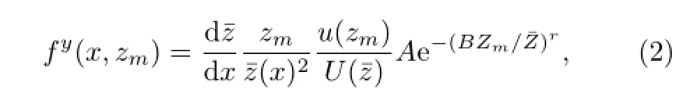
The fyofthe KMmodeltakes into account atmospheric stability and uses the power law profile to calculate the verticalprofile of the eddy diffusivity,K(z), and vertical profile of the wind speed,u(z)(Kormann and Meixner,2001).The final function is

2.2.3 The H model
The fyof the H model uses two similarity constants,D and Q,to reflect atmospheric stability (Hsieh et al.,2000),according to the Gash(1986)footprint model for neutral atmospheric conditions.The final function is

where L is Monin-Obukhov length,K=0.4 is von Karman’s constant,e=2.718,and zuis a length scale that combines zmand z0,i.e.,

The two similarity constants,D and Q,are

2.3 Parameterization
Table 1 shows the initial parameters of the flux footprint for comparison of the three flux footprintmodels.The two measurement heights(zm)are 23.6 and 39.6 m.The measurement height should ensure that the EC is high enough to view the whole study area of interest.The surface distance over which wind has blown is termed fetch,and a rule of thumb,i.e.,the ratio of measurement height and fetch equals 1:100,is generally used.The two surface roughness lengths(z0)are 0.06 and 0.58 m.The Monin-Obukhov length,L,is-158 m for unstable conditions, 165 m for stable conditions,and 14048 m for neutral conditions.Near-neutral conditions are specified for |(zm-d)/L|<0.01 according to Hsieh et al.(2000). Therefore,(zm-d)/L<-0.01 is considered for unstable conditions and(zm-d)/L>0.01 is considered for stable conditions.The three friction velocities(u∗)are 0.48,0.40,and 0.26 m s−1.The three standard deviations of lateral wind fluctuations(σv)are 0.99,0.75, and 0.58.The zero-plane displacement(d)is 8.4 m.

Table 1.Initial parameters for the flux footprints:measurement height zm(m),surface roughness length z0(m), friction velocity u∗(m s−1),standard deviation of lateral wind fluctuationsσv(m s−1),and Monin-Obukhov length L(m)
The source area footprint results from the three models are compared.The variables a(near the end of the source area),i(the far end of the source area), j(the maximum lateralhalf-width of the source area), and Ar(the source area)are the characteristic dimensions of the source area.For the three models,the sensitivity agreement of the source area to(a)measurement height,(b)surface roughness,and(c)atmospheric condition can be assessed through comparing the four characteristic dimensions.The FSAM has been widely adopted but only applied during neutral and moderate atmospheric stability and with a limited range ofcrosswind turbulence intensity(Schmid,2002; Vesala et al.,2008).Therefore,the FSAM results are used as a reference and compared with the other two models.
2.4 Flux footprint climatology
To obtain the flux footprint climatology,the three analytical flux footprint models were run at a 30-min time step,and the data were accumulated to yield seasonal values for each pixel(x,y,zm-z0)separately. The accumulated values of each pixel were normalized by the cumulative seasonal values of the area of interestΩPto yield the flux footprint climatology(Chen et al.,2009),γ(x,y,zm-z0),as
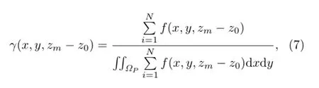
where i is the time step(i.e.,30 min),N is the total number of 30-min periods within a season,andΩPis the area of interest which gives a contribution,P,to the measurement.In implementation of the models, values forγ(x,y,zm-z0)were sorted in a descending order and accumulated from largest to smallest until a given fraction,P,was achieved.Finally,P-level profiles were produced.The calculated flux footprint climatology provides a map of the area around the tower that has contributed to the EC-measured flux.
3.Results
3.1 Comparison of the three flux footprint models
3.1.1 Differences among the three models
Figure 1 illustrates the 90%source areas predictedby the FSAM,KM,and H models at different measurement heights,surface roughness values,and atmospheric conditions.Table 2 shows the values of a,i,j, and Ar of the 90%source area as predicted by the three models at different measurement heights,surface roughness values,and atmospheric conditions.Figure 1 and Table 2 indicate that atmospheric stability is the main factor that has led to differences among the three models.
In neutral and stable conditions,the KM results agree well with the FSAM results.The discrepancies in Ar between KM and FSAM are less than 3%.However,the H results are larger than the FSAM results. In neutralconditions,the discrepancies in Ar between H and FSAM are 4%-11%;whereas in stable conditions,the discrepancies increase to 18%-26%.When the measurement height is 23.6 m with a smooth surface,the discrepancies in Ar between H and FSAM are lowest in neutral conditions and highest in stable conditions.
In unstable conditions,the agreement between the three models is better for a rough surface than for a smooth surface(Fig.1 and Table 2).Additionally,the agreement between the three models for the lower measurement height is better than for the upper measurement height.For smooth surfaces,the Ar magnitude follows the order:KM>FSAM>H;however,for rough surfaces,the order changes to KM>H>FSAM.When the measurement height increases to 39.6 m,the magnitude of results across the three models does not change.Thus,among the models, the differences due to roughness length are larger than those due to measurement height.
3.1.2 Reasons for the differences among the three models
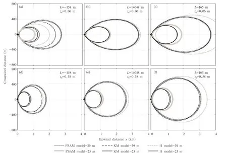
Fig.1.The 90%source areas predicted by the FSAM,KM,and H models at different measurement heights,surface roughness values,and atmospheric conditions.
The footprint differences among the three models originate from the different underlying theories used to construct each model.The FSAM and KM models are theoretical models,whereas the H model is an empiricalmodel.Thus,in Table 3,the FSAMand KMmodels have the same parameters,but these are not shared by the H model.The FSAM and KM models are based on a two-dimensional advection-diffusion equation,or K-theory(Schmid,2002;Foken,2008; Vesala et al.,2008),whereas the H model uses regression analysis to obtain three sets of empirical constants for D and Q in unstable,neutral,and stable conditions(Eq.(6))and forms a footprint model for thermally-stratified atmospheric flows(Hsieh et al., 2000).Therefore,in the present study,when atmospheric stability changes,changes in the H model are larger than those in the other two models.
The discrepancy between FSAM and KM is caused by the same parameter being calculated by different methods(Horst and Weil,1992;Schmid,1994; Kormann and Meixner,2001).Table 3 shows the pa-rameterization methods of the FSAM and KM models.Monin-Obukhov similarity profiles are used in the FSAM model,and power law profiles are used in the KM model.Figure 2 illustrates the differences in the mean plume height for dispersion,effective speed of plume advection(U),gradient ofwith xand shape factor(r)between the FSAM and KM models in neutral conditions when measurement height is 23.6 m and roughness length is 0.58 m.If,U,and r were the same for FSAM and KM,then the results of FSAM and KM would be equal(i.e.,Eq.(2)is equivalent to Eq.(3)),while r is constant in the KM model but variable in FSAM.Differences in the other three parameters between the two models increase with the increasing upwind distance.

Table 2.Values of the variables a,i,j,and Ar of the 90%source area predicted by the FSAM,KM,and H models at different measurement heights,surface roughness values,and atmospheric conditions
Table 3.The parameterization methods for the mean plume height for dispersioneffective speed of plume advection(U),gradient ofwith xand shape factor(r)adopted in the FSAM and KM models
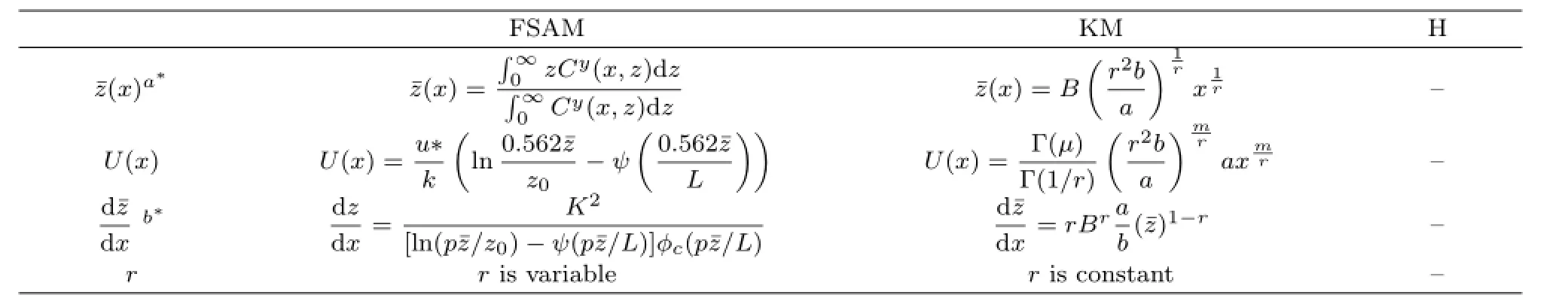
Table 3.The parameterization methods for the mean plume height for dispersioneffective speed of plume advection(U),gradient ofwith xand shape factor(r)adopted in the FSAM and KM models
a*:¯z must be calculated numerically(Horst and Weil,1992).b*:K=0.4 is von Karman’s constant;p=1.55 is also a constant, andψ(p¯z/L)andφc(p¯z/L)are the diabatic integrations of the wind profile and stability function of heat.The specific calculations ofψ(p¯z/L)andφc(p¯z/L)were described by Horst and Weil(1992).Note:a and b are the constants of power laws for the eddy diffusivity and the vertical profile of the horizontal wind velocity,respectively(Kormann and Meixner,2001).The H model,which is empirical,does not use these parameters.
KM H FSAM ?1 ¯z(x)a∗¯z(x)=∫∞0 ?r2 b z Cy(x,z)d z C y(x,z)d z¯z(x)=B ∫∞0 r x1r -U(x)U(x)=u∗? ln 0.562¯z ?? ?0.562¯z U(x)=Γ(μ)?m?r2b a -ψ z0 k L Γ(1/r)araxmr-d¯z b(¯z)1−rr r is variable r is constantb∗d z d¯z d x d x=K2[ln(p¯z/z0)-ψ(p¯z/L)]φc(p¯z/L)d x=rBra
Because the KMresults agree wellwith the FSAM results in stable conditions(Fig.1),the KM and FSAM models can be used equally at night(i.e.,under stable atmospheric conditions).It is considered that the H model should not be used immediately before and after dusk(dawn)when atmospheric stability changes because this causes the H results to change more significantly than the other two models(Fig.1). The discrepancies among the three models could be neglected if the dimension of the study area is sufficiently large.
Based on previous studies,the strength,weakness,and applicability of the three models are reviewed in Table 4.The full version of FSAM is available on the website http://www.indiana.edu/~climate /SAM/SAM−FSAM.html,but some parameters,such as¯z,must be calculated numerically(Horst and Weil, 1992).Therefore,although the FSAM model is expressed by analytical formulae,it can only be evaluated numerically(Schmid,2002).The KM and H models provide analytical solutions because of their mathematical simplicity(Foken,2008).The KM model generally overestimates wind velocity near the ground,especially for unstable conditions and large roughness values(Kormann and Meixner,2001); while,in the present study,a change in atmospheric stability caused the H results to change in an inconsistent manner(Fig.1).The FSAM and KM models are restricted to surface layer scaling conditions due to the Gaussian distribution in the crosswind direction;whereas the H model is applicable to short-term changes in atmospheric stability.

Fig.2.Differences of(a)mean plume height for dispersion,(b)effective speed of plume advection(U),(c)gradient with an upwind distance ofand(d)shape factor(r)between the FSAM and KM models.
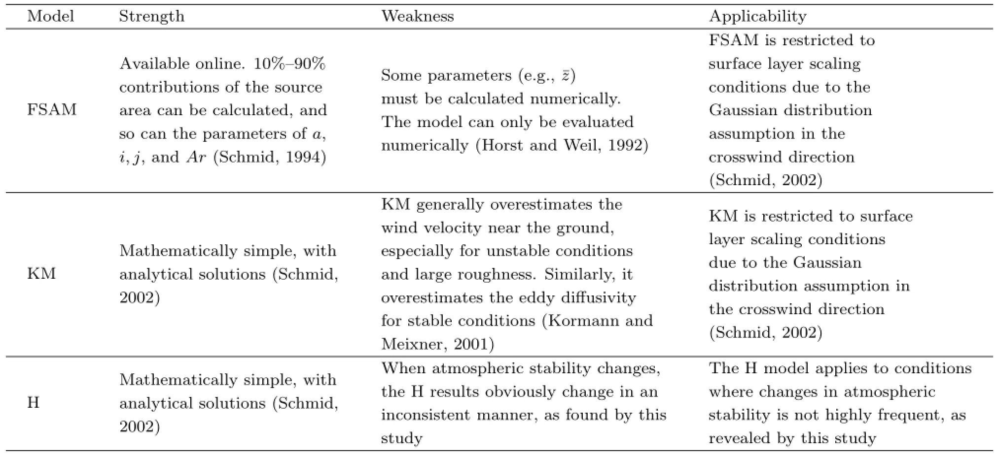
Table 4.Strength,weakness,and applicability of the FSAM,KM,and H models summarized from previous studies and from this study
The conclusions presented in Table 4 are also validated by this study.For example,when atmospheric conditions changed from unstable to stable,the area given by the H model increased by more than double (much more than for the FSAM or KM models)(Fig. 1).When L<0,the size given by the KM model was the largest of the three models(Fig.1).This could be explained by the weakness of the KM model. For example,the KM modeloverestimated wind velocity near the ground,especially for unstable conditions. Because the wind velocity(u(z))was overestimated, the effective speed of plume advection(U)could also have been overestimated(U=u(z)/zm)(Kormann and Meixner,2001)and the EC sensor could access the further source according to the inverted plume assumption(Schmid,2002).In this scenario,the area of the footprint would be overestimated.
3.2 Seasonal variations of the flux footprint climatology
Figure 3 illustrates the seasonal variations of the flux footprint climatology as predicted by the three models for receptor locations at two and three times the canopy height.For clarity,the corresponding wind directions are also shown.There are similar seasonal patterns in the flux footprint climatologies assessed by the three models.
The seasonal flux footprint climatologies are distributed asymmetrically around the tower and correspond well to the prevailing wind direction.In 2003, the 90%flux footprint climatologies of the three models at 23.6 m were 27%-29%from the north-northwest part of the receptor and 26%-28%from the southsoutheast part of the receptor.In summer,the flux footprint climatology in the south-southeast region increased to 51%.In autumn,the main distribution of the flux footprint climatology returned to the northnorthwest where 38%-52%contributed to the receptor.In winter,a 33%-50%contribution also originated from the north-northwest.The distributions of the flux footprint climatologies at 39.6 m were similar to those at 23.6 m.From spring to winter,the contribution of the north-northwest part at 39.6 m was 5% less than that at 23.6 m,but the contribution of the south-southeast part did not significantly change.
The average sizes of the 90%flux footprint climatologies of the three models in 2003 for the receptor at 23.6 m were 0.61-0.74 km2in spring,0.45-0.67 km2in summer,0.38-0.42 km2in autumn,and 0.36-0.69 km2in winter.The seasonalaverage sizes followed the order:spring>summer>winter>autumn,whereas the seasonal changes in the sizes followed the order:winter>summer>autumn>spring.The sizes for the receptor at 39.6 m were on average 4.6 times larger than those at 23.6 m.The sizes were 2.69-3.19 km2in spring,2.07-3.28 km2in summer,1.74-2.36 km2in autumn,and 1.54-2.90 km2in winter.The difference between the two measurement heights did not change significantly with season.
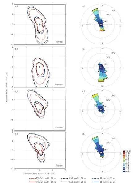
Fig.3.Seasonal variations of the flux footprint climatologies(left panels)simulated by FSAM(red),KM(black), and H(blue)models at 23-(solid)and 39-m(dotted)measurement heights,and the corresponding wind rose diagrams (right panels),for(a1,a2)spring,(b1,b2)summer,(c1,c2)autumn,and(d1,d2)winter over the subtropical coniferous plantation in Southeast China.The tower position was located at(0,0).
4.Discussion
4.1 Effect of atmospheric stability on flux footprint climatology
Footprint climatologies depend on atmospheric stability on a daily scale.For example,Chen et al. (2008)revealed that the flux footprint area in the daytime was smaller than that at nighttime because more unstable conditions occur during daytime and more stable conditions occur at night.During stable conditions,the measurements can be affected by turbulence characteristics of the vertical wind velocity from further upwind(G¨ockede et al.,2006;Foken,2008).
However,footprint climatologies less clearly depend on atmospheric stability on a seasonalscale.Figure 4a shows the linear regression(R2=0.38)between the size of flux climatology and the frequency of a stable atmosphere.Atmospheric stability varied for a short time;therefore,its influence on footprint climatologies was weaker for continuous observations over long periods.
4.2 Effect of the standard deviation of lateral wind fluctuations on flux footprint climatology
Figure 4b shows the linear regression(R2=0.73) between the size of flux climatology and the standard deviation of lateral wind fluctuations.The size of the flux footprint climatology increased with the increasing standard deviation of the lateralwind fluctuations. In Eq.(1),the crosswind dispersion,Dy,is generally assumed to be Gaussian(Horst and Weil,1992),

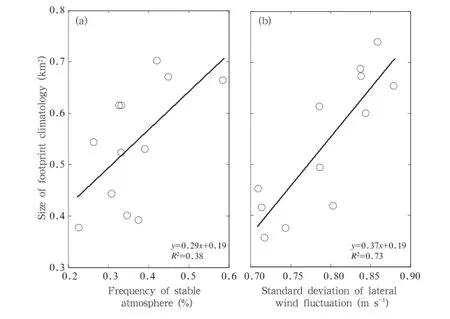
Fig.4.Linear regression between the size of flux climatology and the(a)frequency of stable conditions and(b)standard deviation of the lateral wind fluctuations.
4.3 Effect of measurement height on flux footprint climatology
The results in this study showed that the size of the flux footprint climatology could be increased by three-fold when the measurement height increased to twice the canopy height(Fig.3).The majority of current footprint models rely,either implicitly or explicitly,on the inverted plume assumption(Schmid, 2002).The mean plume height(¯z)and the effective speed of plume advection(U)which are characteristic parameters of plumes,depend on the measurement height according to the equations in Table 3(Horst and Weil,1992).Figure 5 illustrates the effect of measurement height on¯z and U.Variables¯z and U were the results of the FSAM model for an unstable condition.When the measurement height increased,the mean plume height,¯z,also increased and the effective speed of the plume advection,U,decreased;therefore, turbulence may have been received from a more distant source area(Aubinet et al.,2012).Therefore,the EC sensors should be high enough to access the environment through,and above,the main plant canopy of interest(Aubinet et al.,2012).
5.Conclusions
In this study,we elucidated the seasonal variations of flux footprint climatologies and the major factors that influence them using the analytical FSAM, KM,and H models based on eddy covariance measurements at two and three times the canopy height at the Qianyanzhou site of ChinaFLUX.
A comparison of the three analytical models demonstrated that atmospheric stability was the main factor that led to differences among the three models on a daily scale.In neutral and stable conditions, the KM results agreed well with the FSAM results, whereas the H results were larger than the KM and FSAM results.In unstable conditions,the agreement among the three models for rough surfaces was better than that for smooth surfaces.Further,the lower measurement height(23.6 m)produced better agreement than the upper measurement height(39.6 m).The differences due to roughness length were larger than those due to measurement height.The differences in footprints among the three models were caused by the different underlying theories used to construct each model.The FSAM and KM models are theoreticalmodels,whereas the H model is empirical.

Fig.5.The effect of measurement height on(a)mean plume height(m)and(b)effective speed of plume advection(m s−1).
The FSAM model is available online,but some parameters,such as¯z,must be calculated numerically. The KM and H models provide analytical solutions because of their mathematical simplicity.The KM model generally overestimates wind velocity near the ground,especially for unstable conditions and large roughness values.When atmospheric stability varies, the H results change in an inconsistent manner.Because the FSAM and KM models both assume Gaussian distributions in the crosswind direction,and all the parameters ofthe two models are expressed for surface layer,these models are restricted to surface layer scaling conditions.The present study reveals that the H model is applicable to low-frequency changes in atmospheric stability.
This study found that the seasonal flux footprint climatologies were distributed asymmetrically around the observation tower and corresponded well to the prevailing wind direction.The predominant distributions were north-northwest in winter and southsoutheast in summer.The average sizes of the 90% flux footprint climatologies were 0.36-0.74 and 1.5-3.2 km2at two and three times the canopy height,respectively.The seasonal average sizes followed the order: spring>summer>winter>autumn.
The footprint climatologies clearly depended on the atmospheric stability on daily scale,but less clearly on seasonal scale.This was because atmospheric stability is only variable for a short time, and its influence on footprint climatologies is weaker for continuous observations over long periods.The size of the flux footprint climatology increased as the standard deviation of the lateral wind fluctuations increased and,therefore,crosswind dispersion increased.The flux footprint climatology increased three-fold when the measurement height increased to twice the canopy height.
Acknowledgments.We thank Dr.Schmid for providing the source code of the FSAM model online.
REFERENCES
Allen,R.G.,L.S.Pereira,T.A.Howell,et al.,2011: Evapotranspiration information reporting.I:Factors governing measurement accuracy.Agr.Water Manage.,98,899-920.
Amiro,B.D.,1998:Footprint climatologies for evapotranspiration in a boreal catchment.Agr.Forest. Meteor.,90,195-201.
Aubinet,M.,T.Vesala,and D.Papale,2012:Eddy Covariance:A Practical Guide to Measurement and Data Analysis.Springer,New York,21-58 pp.
Baldocchi,D.D.,2008:“Breathing”of the terrestrial biosphere:Lessons learned from a global network of carbon dioxide flux measurement systems.Aust.J. Bot.,56,1-26.
Biermann,T.,W.Babel,E.Thiem,et al.,2011:Energy fluxes above Nam Co Lake and the surrounding grassland—The NamCo 2009 experiment.7th Sino-German Workshop on Tibetan Plateau Research,Hamburg,Germany,3-6 March,German TiP project and Institute of Tibetan Plateau Research.
Cai,X.H.,J.Y.Chen,and R.L.Desjardins,2010: Flux footprints in the convective boundary layer: Large-eddy simulation and lagrangian stochastic modelling.Bound.-Layer Meteor.,137,31-47.
Cai,X.H.,M.J.Zhu,S.M.Liu,et al.,2011:Flux footprint analysis and application for the large aperture scintillometer.Adv.Earth.Sci.,25,1166-1174.
Chen,B.,Q.Ge,D.Fu,et al.,2010:A data-model fusion approach for upscaling gross ecosystem productivity to the landscape scale based on remote sensing and flux footprint modelling.Biogeosciences,7,2943-2958.
Chen,B.Z.,J.M.Chen,G.Mo,et al.,2008:Comparison of regional carbon flux estimates from CO2concentration measurements and remote sensing based footprint integration.Global Biogeochem.Cycle,22,doi:10.1029/2007GB003024.
Chen,B.Z.,N.C.Coops,D.J.Fu,et al.,2011:Assessing eddy-covariance flux tower location bias across the fluxnet-Canada research network based on remote sensing and footprint modelling.Agr.Forest Meteor.,151,87-100.
Chen,B.Z.,N.C.Coops,D.J.Fu,et al.,2012:Characterizing spatial representativeness of flux tower eddy-covariance measurements across the Canadian carbon program network using remote sensing and footprint analysis.Remote Sens.Environ.,124, 742-755.
Chen,B.Z.,T.A.Black,N.C.Coops,et al.,2009:Assessing tower flux footprint climatology and scaling between remotely sensed and eddy covariance measurements.Bound.-Layer Meteor.,130,137-167.
Foken,T.,2008:Micrometeorology.Springer-Verlag, Berlin,Heidelberg,82-87.
Gash,J.H.C.,1986:A note on estimating the effect of a limited fetch on micrometeorological evaporation measurements.Bound.-Layer Meteor.,35,409-413.
Horst,T.W.,and J.C.Weil,1992:Footprint estimation for scalar flux measurements in the atmospheric surface layer.Bound.-Layer Meteor.,59,279-296.
Hsieh,C.I.,G.Katul,and T.W.Chi,2000:An approximate analytical model for footprint estimation of scalar fluxes in thermally stratified atmospheric flows.Adv.Water Resour.,23,765-772.
Kljun,N.,2010a:Attributing tall tower flux data to heterogeneous vegetation.19th Symposium on Boundary Layers and Turbulence,Keystone,Colorado,2-6 August,Amer.Meteor.Soc.
Kljun,N.,2010b:BERMS sites revisited:Footprint climatology and 3D-LiDAR data.29th Conference on Agricultural and Forest Meteorology,Keystone, Colorado,2-6 August,Amer.Meteor.Soc.
Kormann,R.,and F.X.Meixner,2001:An analytical footprint model for non-neutral stratification. Bound.-Layer Meteor.,99,207-224.
Leclerc,M.Y.,and G.W.Thurtell,1990:Footprint prediction of scalar fluxes using a Markovian analysis. Bound.-Layer Meteor.,52,247-258.
Leclerc,M.Y.,and T.Foken,2014:Footprints in Micrometeorology and Ecology.Springer-Verlag, Berlin,Heidelberg,71-98.
Leuning,R.,2005:Measurements of trace gas fluxes in the atmosphere using eddy covariance:WPL corrections revisited.Handbook of Micrometeorology:A Guide for Surface Flux Measurement and Analysis. Springer,Netherlands,119-132.
Rebmann,C.,M.Gockede,T.Foken,et al.,2005:Quality analysis applied on eddy covariance measurements at complex forest sites using footprint modeling. Theor.Appl.Climatol.,80,121-141.
Schmid,H.P.,1994:Source areas for scalars and scalar fluxes.Bound.-Layer Meteor.,67,293-318.
Schmid,H.P.,2002:Footprint modeling for vegetation atmosphere exchange studies:A review and perspective.Agr.Forest Meteor.,113,159-183.
Sogachev,A.,and J.Lloyd,2004:Using a one-and-a-half order closure model of the atmospheric boundary layer for surface flux footprint estimation.Bound. -Layer Meteor.,112,467-502.
Tang,Y.K.,X.F.Wen,X.M.Sun,et al.,2014a:The limiting effect of deep soilwater on evapotranspiration of a subtropical coniferous plantation subjected to seasonaldrought.Adv.Atmos.Sci.,31,385-395.
Tang,Y.K.,X.F.Wen,X.M.Sun,et al.,2014b:Interannual variation of the bowen ratio in a subtropical coniferous plantation in Southeast China, 2003-2012.Plos One,9,e88267,doi:10.1371/journal.pone.0088267.
Webb,E.K.,G.I.Pearman,and R.Leuning,1980:Correction of flux measurements for density effects due to heat and water vapour transfer.Quart.J.Roy. Meteor.Soc.,106,85-100.
Wen,X.F.,G.R.Yu,X.M.Sun,et al.,2006:Soil moisture effect on the temperature dependence of ecosystem respiration in a subtropical Pinus plantation of southeastern China.Agr.Forest Meteor.,137,166-175.
Wen,X.F.,H.M.Wang,J.L.Wang,et al.,2010: Ecosystem carbon exchanges of a subtropical evergreen coniferous plantation subjected to seasonal drought,2003-2007.Biogeosciences,7,357-369.
Wilczak,J.M.,S.P.Oncley,and S.A.Stage,2001:Sonic anemometer tilt correction algorithms.Bound. -Layer Meteor.,99,127-150.
Yu Guirui,Wen Xuefa,and Sun Xiaomin,et al.,2006: Overview of ChinaFLUX and evaluation of its eddy covariance measurement.Agr.Forest Meteor.,137, 125-137.
Zhang Hui,Shen Shuanghe,Wen Xuefa,et al.,2012:Flux footprint of carbon dioxide and vapor exchange over the terrestrialecosystem:A review.Acta Ecol.Sin.,32,7622-7633.(in Chinese)
Zhang Huiand Wen Xuefa,2015:Flux footprint climatology estimated by three analyticalmodels over a subtropical coniferous plantation in Southeast China.J.Meteor.Res.,29(4),654-666,
10.1007/s13351-014-4090-7.
Supported by the National Basic Research and Development(973)Program of China(2012CB416903),National Natural Science Foundation of China(31470500 and 31290221),and Knowledge Innovation Project of the Chinese Academy of Sciences (KZCX2-EW-QN305).
∗wenxf@igsnrr.ac.cn.
©The Chinese Meteorological Society and Springer-Verlag Berlin Heidelberg 2015
February 6,2015;in final form June 16,2015)
猜你喜欢
教育家(2022年17期)2022-04-23
美与时代·城市版(2022年1期)2022-03-05
校园英语·上旬(2019年8期)2019-09-16
饮食科学(2018年3期)2018-06-01
美与时代·美术学刊(2018年3期)2018-04-30
新高考·高二数学(2017年3期)2017-08-17
美与时代·美术学刊(2017年6期)2017-07-31
新高考·高二数学(2016年3期)2016-05-20
东南大学学报(医学版)(2015年2期)2015-03-22
中国篆刻·书画教育(2014年1期)2014-03-10
 Journal of Meteorological Research2015年4期
- Journal of Meteorological Research的其它文章
- Regional Warming by Black Carbon and Tropospheric Ozone: A Review of Progresses and Research Challenges in China
- Comprehensive Radar Observations of Clouds and Precipitation over the Tibetan Plateau and Preliminary Analysis of Cloud Properties
- The Key Oceanic Regions Responsible for the Interannual Variability of the Western North Pacific Subtropical High and Associated Mechanisms
- Underestimation of Oceanic Warm Cloud Occurrences by the Cloud Profiling Radar Aboard CloudSat
- Performance of CMIP5 Models in the Simulation of Climate Characteristics of Synoptic Patterns over East Asia
- Nonlinear Responses of Oceanic Temperature to Wind Stress Anomalies in Tropical Pacific and Indian Oceans:A Study Based on Numerical Experiments with an OGCM