
Modeling the Middle Jurassic ocean circulation
2015-03-21 05:49MurBrunettiChristinrrdPeterBumgrtner
Journal of Palaeogeography 2015年4期
Mur Brunetti *, Christin Vérrd Peter O. Bumgrtner
a Institute for Environmental Sciences, University of Geneva, Bd Carl-Vogt 66, CH-1205
Geneva, Switzerland
b Institute of Earth Sciences, University of Lausanne, Géopolis, CH-1015 Lausanne, Switzerland
1 Introduction
Earth’s climate is a complex system which evolves under the action of internal dynamics of highly coupled subsystems (ocean, atmosphere, ice masses, land surface,etc.) and external factors (Saltzman, 2002; and references therein), such as the astronomical forcing (changes in solar luminosity, Earth’s orbit and tilt) and the tectonic forcing(plate tectonics, volcanic activity). We are interested in investigating how the ocean circulation (whose relaxation time is of the order of 100-1000 years) responds to changes in plate tectonic setting of ocean basins and land masses(which act on very long time-scales of the order of 10 My).Given the large difference between the ocean and tectonic time-scales, the tectonic forcing can be considered as a constant during the ocean response time and we look for equilibrium states of ocean currents for given different tectonic configurations. This method allows us to find the main regions of upwelling and downwelling (where organic activity is maximum), anoxic regions (e.g., stagnant circulation caused by the presence of barriers to deep circulation),overturning cells and gyre patterns for a given geological period, and to evaluate the model results against palaeoclimate records.
We use an ocean general circulation model (OGCM) coupled to the sea-ice component, while the contributions of other internal subsystems, which affect the interface between the ocean and the atmosphere and can be described by fast-response variables, are included as specified monthly averaged boundary conditions at the ocean surface. This is a first-order approximation which does not account for possible feedbacks between the averaged components and the dynamical ones, and which reduces internal variability.We will relax this approximation in further studies.
In this paper, we present the results of global oceansea-ice simulations conducted using the Massachussetts Institute of Technology (MIT) general circulation model (Marshallet al., 1997a, 1997b). For this first study, we have chosen the Middle Jurassic (Callovian) Epoch (~165 Ma). We plan to investigate other geological intervals in a systematic way by applying the methods discussed in the present paper. A main improvement with respect to previous studies of the Jurassic ocean circulation (Bjerrumet al., 2001;Dera and Donnadieu, 2012) is the bathymetry model, which is based on reconstructions of oceanic realms, in particular of Panthalassa (Flores-Reyes, 2009; Vérardet al., 2015a,2015b; and see section 2).
The Callovian-Oxfordian transition is an interesting geological period since it records perturbations in the carbonate deposition pattern and cooling of seawater temperature whose causes are still debated (Donnadieuet al., 2011). Pangaea breakup started in the Early Jurassic by rifting between Laurasia and Gondwana, resulting in the formation of the Central Atlantic and its connection with the Neo-Tethys (see Fig. 1). While an Early Jurassic(Toarcian) opening of the Central Atlantic is now well constrained (e.g., Knelleret al., 2012; Labailset al., 2010),rifting and breakup between North and South America is still controversial. A number of plate tectonic models place the Proto-Caribbean breakup in the Early Jurassic (e.g.,Stampfli and Borel, 2004), while others opt for prolonged crustal extension between the Americas and breakup by the early Late Jurassic (e.g., Pindell and Kennan, 2009). A first marine Proto-Caribbean passage may have been opened in the Middle Jurassic, but the oldest clearly Proto-Caribbean ocean crust is only of early Late Jurassic age (Baumgartner,2013; Pindell and Kennan, 2009). Here, we examine both the configurations with and without an open connection between the Proto-Caribbean and Panthalassa.
In the literature, several examples of comparisons between the results of atmospheric general circulation models(AGCM) and geological and phytogeographical data can be found for the Jurassic (Mooreet al., 1992; Sellwood and Valdes, 2008; Sellwoodet al., 2000; Valdes, 1993). In these papers, ocean dynamics are not included explicitly or described by simplified models, such as mixed layer models(Mooreet al., 1992), since the aim was to find the dynamical equilibrium between the atmosphere and a given orography. In the present paper, we will discuss the results of numerical simulations that explicitly follow ocean dynamics.

Figure 1 Palaeo-Digital Elevation Model of the Earth at ~165 Ma applied on the plate tectonic model developed at the University of Lausanne (UNIL) (© Shell Global Solutions International, 2013; version 2010 of the UNIL Plate Model). Abbreviations are: NAm: North America;SAm: South America; Ant: Antarctica; Aus: Australia; G: Greenland; I: Iberia; A: Adria; T: Taurus; AT: Alpine Tethys; BN: Bangong-Nujiang;ES: Elise Sea. Mollweide projection.
The role of the ocean in Jurassic climates has been investigated in the past (Chandleret al., 1992; Rind and Chandler, 1991). The ocean has been found to be an important dynamical component, the treatment of which likely explains different model predictions, in particular at high latitudes. Typically, atmospheric CO2concentrations in the Jurassic are taken to be between 1 and 7.5 times pre-industrial values (Mooreet al., 1992; Reeset al., 2000; Sellwood and Valdes, 2008; Valdes, 1993). The effect of increased concentrations of CO2in the atmosphere is to warm tropical regions as well as high latitudes. In order to obtain a reduced meridional temperature gradient, which is characteristic of warm climates, different mechanisms need to be considered. Since Jurassic simulations with specified seasurface temperatures warmer than the present-day values were found in energy balance without requiring high atmospheric CO2concentrations (Chandleret al., 1992), it was suggested that warm Jurassic climates can be produced by enhanced poleward heat transport through the ocean.This hypothesis has, however, been questioned by Late Jurassic simulations with a specified, reduced meridional sea-surface gradient. These simulations indeed show that the required ocean heat transport is much smaller than in present-day simulations (Valdes, 1993).
A possible physical mechanism for reproducing the reduced meridional temperature gradient of warm climates and at the same time increasing poleward ocean heat transport is the existence of a low-latitude circum global passage during the Mesozoic and Early Cenozoic (Hotinski and Toggweiler, 2003). However, a Tethyan circum global passage has the effect of driving high rates of upwelling which is not confirmed by recent analysis of Middle Jurassic deep-sea sediments (Baumgartner, 2013). Moreover, previous studies of the ocean circulation during the Cretaceous have shown that the Tethyan circum global current and water properties are sensitive to bathymetry (Bush, 1997;Poulsenet al., 2003). In this paper, we address these open issues.
The paper is organized as follows: In section 2, we describe the plate tectonic model. In section 3, we summarise recent results on Middle Jurassic sediments, in particular in the Central Atlantic and the Proto-Caribbean basin. In section 4, we describe the MIT general circulation model together with the parameters and the boundary conditions at the ocean surface used in the numerical experiments.Section 5 shows the simulation results and compares them to geological records. Finally, section 6 includes our summary and conclusions.
2 Palaeo-Digital Elevation Model (DEM) and the underlying plate tectonic reconstruction
Plate tectonic processes act on a time scale of tens of million years and modify the size and distribution of continents inducing changes in atmospheric and oceanic circulation patterns, thus giving rise to climatic changes on such a long time scale (Barron, 1981).
The plate tectonic model that we use in the present study is a part of the model owned by Shell Global Solutions International, and it is based on the 2010 version of the model developed at the University of Lausanne (UNIL)for more than 20 years (readers are referred to numerous publications, among which, Ferrariet al., 2008; Hochard,2008; Moixet al., 2008; Stampfli, 2013; Stampfli and Borel,2002, 2004; Stampfli and Kozur, 2006; Stampfliet al., 2013;Vérard and Stampfli, 2013a, 2013b; Vérardet al., 2012;vonRaumeret al., 2006; Wilhem, 2010). This model reconstructs the evolution of the Earth surface from 600 Ma to present. It is the sole model hitherto to cover 100% of the Earth surface over such a long time interval, and the approach employed allows reconstruction of not only continental areas but also oceanic realms, and in particular ocean domains that have since subducted. The model follows plate tectonic rules, meaning that it is coherent with scenarios figured at lithospheric scale, physically coherent with forces acting at plate boundaries, and overall, deeply rooted in geological information.
On top of it, we have developed a heuristic-based method (Vérardet al., 2015a, 2015b) to convert geodynamical models in three dimensions (3D),i.e., creating synthetic reliefs (hypsometry and bathymetry). For this purpose,a novel code has been developed under ArcGIS® and applied to the plate tectonic model owned by Shell (© Shell Global Solutions International, 2013; version 2010 of the UNIL plate tectonic model). Contrary to other tentatives to produce palaeo-Digital Elevation Model (DEM),e.g., DEM used in Donnadieuet al., 2006; Markwick and Valdes, 2004;Nardinet al., 2011; Roscheret al., 2011; and Sellwood and Valdes, 2006, this 3D conversion allows flooding of continental areas which have their own relief and compute synthetic sea-level and coast lines. The version used herein has been tested against independent datasets (e.g., tomography; Hafkenscheidet al., 2006; Webb, 2012) and has revealed satisfactory results in retrieving long-term variations of different palaeoclimate indicators (Vérardet al.,2015a, 2015b). Although more sophisticated 3D modeling is needed in the future, such an approach to convert 2D maps into 3D has the advantage to be applicable anywhere on the globe and at any geological time.
We thus produced a full global palaeo-DEM for the Callovian (~165 Ma) with a resolution of 0.1°. From West to East,the main features that may have an impact on global water circulation are as follows (Fig. 1):
1) Following Pangaea break-up, most of the landmass is gathered in one hemisphere; the rest is represented by the Panthalassa Ocean, which covered 165° of longitude. The Panthalassa Ocean is delimited on its western side from the Neo-Tethys by a largely transtensive mid-oceanic spreading axis, with relief of 2500 m above surrounding abyssal plains oriented perpendicularly to general water circulation.
2) In the middle of the Panthalassa Ocean, and in the domain of equatorial currents, the nascent Pacific Ocean is bounded by high relief features corresponding to trenches and island arcs forming a triangular zone.
3) In the Arctic domain, the Selwyn Sea (named after the Selwyn Basin, Yukon;e.g., Stampfliet al., 2013) is a vast area surrounded by continental crust, and therefore relatively closed.
4) The palaeogeography of the young Central Atlantic and Proto-Caribbean is essential in the modeling of the Middle Jurassic ocean circulation, as it is E-W-oriented.The question is whether a circum-global current may have flown through it (Hotinski and Toggweiler, 2003; Iturralde-Vinent, 2006). However, important bottlenecks exist to the East (shallow gateway between Iberia and North Africa) and to the West (Florida Promontory, Bahamas Hotspot, and a shallow passage documented by evaporites). West of the Proto-Caribbean basin, a major bottleneck may have existed until the Late Jurassic/earliest Cretaceous between Yucatan and South America due to a strike slip movement(Flores-Reyes, 2009) or an oblique spreading ridge (Pindellet al., 2012) between the two continental blocks. Although the palaeo-DEM does not take dynamic topography into account, the proposed shallow water environment of the plateau is in agreement with coeval evaporatic deposits.
5) The geological complexity of the Adria-Taurus-Vardar domain (Fig. 1) has been extensively studied (e.g., Moixet al., 2008; Stampfli and Kozur, 2006; among many others).However, one of the caveats concerning the 3D conversion is that stretching or shortening is modelled in ‘tectonically identified’ areas such as rifts or collision zones, but not as ‘diffuse regions’, as can be exemplified by the presentday Lord Howe Rise or Falkland Plateau, for instance (such improvement is currently under progress). Consequently,although thermal subsidence of passive margins, in particular, is taken into account (meaning that rift shoulders may go under sea level through time), most of the Adria-Taurus area is emergent in the palaeo-DEM. Yet, geological evidence suggests that the entire domain was more or less stretched and under shallow marine water conditions in the Callovian (Baumgartner, 2013,op. cit.Fig. 6B).
6) Likewise, the synthetic topography and associated sea level suggests that there was no connection between the Arctic Ocean and the Atlantic in the Callovian. Although under-estimated stretching and/or dynamic topography might distort this result regarding water connectivity, we regard, on the basis of the computed palaeo-DEM, major flux between the two basins as unlikely.
7) The last specific feature of the Callovian palaeo-DEM that we wish to point out herein is the presence of the Elise Sea (ES in Fig. 1; see also Vérard and Stampfli, 2013b), a back-arc that developed east of Australia. The location of the Elise Sea is prominent because it is just at the limit between the opened Austral Ocean and the Panthalassan gyre in the southern hemisphere.
3 Deep-sea sediments
The early evolution and the initial breakup history of Pangaea, in particular in the Proto-Caribbean basin, are still debated. In this section we summarise the main constituents of deep-sea sediments in the Middle Jurassic.
Biosiliceous sediments mainly derived from radiolarians dominate the open ocean sedimentary record of Panthalassa and Tethys throughout the Jurassic, suggesting medium to high surface fertility conditions (Baumgartner, 2013). In the Jurassic Central Atlantic and Proto-Caribbean, however, radiolarites are unknown. Ocean drilling in the Central Atlantic has revealed either clay-rich or calcareous Jurassic sediments, and outcrops assigned to the Proto-Caribbean margin and initial oceanic basin of NE Cuba are dominated by carbonates (Iturralde-Vinent and Pszczólkowski, 2011).The pelagic carbonates had two sources: (1) peri-platform ooze shed by carbonate platforms bordering the narrow Central Atlantic and the Proto-Caribbean, such as the Bahamas, Florida and Yucatan; and (2) calcareous nanoplankton, which were scarce in the Middle Jurassic, but became increasingly important after the Oxfordian (Ceccaet al.,2005).
Mass productivity of Nanoconids since the latest Jurassic has been related to oligotrophic conditions in the Central Atlantic (Erba, 1994). The presence of pelagic carbonates in the Jurassic Central Atlantic and the Proto-Caribbean throughout the Jurassic and the Early Cretaceous can be interpreted as the consequence of surface waters that are more oligotrophic than those of the adjacent Tethys and Panthalassa. The Jurassic Central Atlantic was likely similar to a Mediterranean ocean basin such as the modern Red Sea (Baumgartner, 2013). Thus, the distribution of deep-sea sediments seems to exclude a vigorous equatorial trans-Pangaean current through the Central Atlantic-Proto-Caribbean, which would allow mixing of nano-fossil population (Baumgartner, 2013). We will test the presence of this current through numerical ocean-circulation experiments,as described in the following sections.
4 Ocean model and experimental setup
Our numerical experiments have been conducted using the MIT general circulation model (Marshallet al., 1997a,1997b),i.e., a three-dimensional (3D) global model that can be run using a variety of curvilinear coordinates (see the documentation at http://mitgcm.org). For our study,we use the cubed-sphere grid (Adcroftet al., 2004). Since this curvilinear coordinate system avoids Pole singularities,it allows us to properly describe the Polar regions, and in particular the South Pole, which was covered by Panthalassa Ocean during the Middle Jurassic (Fig. 1).
In the absence of ocean-atmosphere feedbacks, our uncoupled modeling approach only allows us to look at largescale responses of ocean circulation to different surface forcing or bathymetry.
We use a time-step of∆t= 1800 s and we perform synchronous runs (Danabasoglu, 2004). In the fine resolution cs64 runs, we modified sub-grid parameterisations (Table 1)in order to avoid instabilities. In particular, in the fine resolution cs64 runs, a biharmonic viscosity (instead of Laplacian viscosity) is used and the vertical mixing diffusion is computed by the so called K-profile parameterisation (kpp package), which unifies the treatment of a variety of unresolved processes involved in vertical mixing (Largeet al., 1994).Thus different small-scale processes are at play in cs32 and cs64 runs and the results of these simulations cannot directly be compared. The MIT model includes the Gent-McWilliams parameterisation of eddies (gmredi package) (Gent and McWilliams, 1990). The parameters used in the ocean circulation experiments are summarized in Table 1.
We compare the results of two different sea-ice models (see Table 2, fourth column). The first is a simple parameterisation where water with a potential temperature less thanθF= -1.9°C is converted into ice which floats at the surface without heat release (this model is denoted by‘freezing’ in Table 2). The second is a dynamical sea-ice model which computes ice thickness, ice concentration and snow cover (Zhang and Hibler, 1997). Parameters for the sea-ice package (e.g., ice/snow albedos and drag coeffi-cients) are taken from present-day simulations with similar resolutions.
The simulations are initialized from rest. Initial threedimensional distributions of potential temperature and salinity are derived from Levitus and Boyer annual fields(Levitus and Boyer, 1994) by taking the zonal average over the present-day Pacific Ocean, as described in the following part for the forcing fields. We begin the simulations without snow and without ice covered oceans. The model is integrated for 300-1000 years (see Table 2, third column),which is of the order of the ocean relaxation time, and the last 30 model years are used for diagnostics.
Forcing fields
A critical aspect of palaeoclimate modeling is to accurately define the boundary conditions for a past age where geological reconstructions are affected by sparsity of data and large uncertainty (Saltzman, 2002). We have adopted the following simplifications.
During the Middle Jurassic, there was one principal ocean with dynamical features probably similar to the present-day Pacific Ocean. Thus, we derive the Jurassic surface forcings from the present-day fields, zonally averaged over the Pacific Ocean. In particular, the atmospheric surface forcings are constructed from the NCEP/NCAR Rea-nalysis monthly means (Kalnayet al., 1996) and they vary throughout the year reproducing the seasonal cycle.
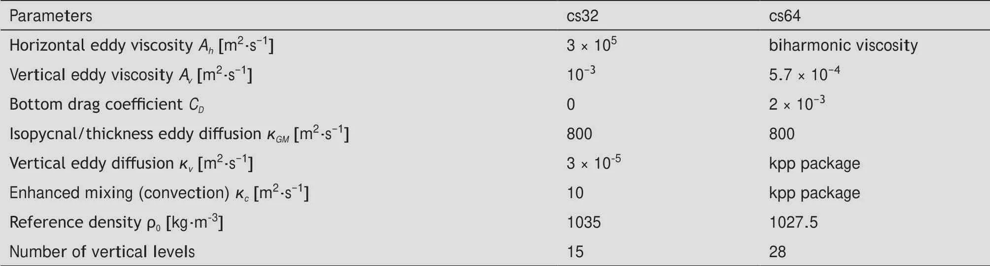
Table 1 Parameters used in the ocean circulation experiments for the cubed sphere configuration with 32 × 32 and 64 × 64 points per face of the cube, denoted respectively by cs32 and cs64
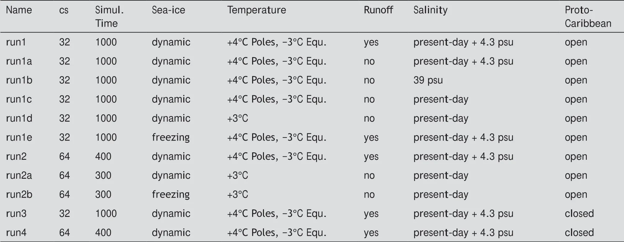
Table 2 List of numerical experiments
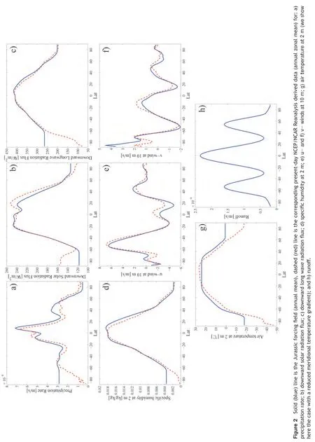
Since the Jurassic Polar regions were warmer and wetter than the present ones (as suggested by proxies, such as those published by Prokophet al.(2008)), we set values at highest north and south latitudes equal to those at 70N and 65S, respectively. These two approximations (zonal average over the Pacific Ocean and correction at high latitudes) have been applied to the following surface forcing fields: precipitation rate, specific humidity at 2 m, downward short-wave and long-wave radiation flux (Fig. 2). For the surface winds we apply only the first approximation.For comparison, modern winds and salt flux estimates were used in the past for modeling warm climates as the Jurassic (Hotinski and Toggweiler, 2003). The solar constant, all orbital constants and input parameters (apart from sea surface temperature and ocean heat flux) were kept at their present-day values in previous studies of Mesozoic climates with AGCMs (Mooreet al., 1992; Sellwood and Valdes, 2008;Sellwoodet al., 2000; Valdes, 1993).
乔治·桑:生活中的某个时刻,我们争取幸福、获得信任、感受陶醉的能力达到顶点。接下来,疑虑与忧郁就笼罩上来,并把我们永远裹住,就好像我们的灵魂不能再满足它们的需求。或许这就是其实正在黯然隐去的命运,我们被判定要缓缓地步下曾经乘兴勇敢地攀上的高坡。
In the last two panels of Figure 2, we show the 2 m air temperature and the runoff, which have been constructed in a different manner. We have corrected the present-day temperatures in two different ways: (1) the air temperatures are uniformly increased by 3°C with respect to present-day values to mimic the effects of higher CO2concentrations in the atmosphere; (2) the air temperatures are increased by 4°C at the Poles and decreased by 3°C at the tropics, in order to reproduce the reduced meridional temperature gradient typical of warm climates (Prokophet al., 2008; Valdes, 1993). We have run simulations with both types of forcing, as listed in Table 2, fifth column. We obtain in such a way a global annual-averaged air temperature at 2 m of 18.2°C for case (1) (uniformly increased temperatures) and of 16.6°C for case (2) (reduced meridional temperature gradient). For comparison, the present-day annual-average calculated from the NCEP/NCAR Reanalysis monthly mean in the period 1981-2010 is 14°C.
The order of magnitude and the qualitative behaviour(for example the asymmetry between the air temperatures of the two hemispheres) of the assumed Jurassic forcing fields compare reasonably well with the output of AGCMs for Jurassic climates over the ocean (see Mooreet al.,1992; Sellwood and Valdes, 2008; Sellwoodet al., 2000;Valdes, 1993 for the Late Jurassic for example; and Reeset al., 2000 for the Jurassic) and of AOGCMs (Dera and Donnadieu, 2012).
The runoff is related to the centres of heavy precipitation and it is essentially concentrated to the Jurassic Neo-Tethys (Mooreet al., 1992). We have derived the runofffrom data in François and Walker (1992), which have been symmetrized and averaged with respect to the Equator. The result is shown in the last panel of Figure 2. We have run simulations with and without this forcing field, as shown in
Table 2, sixth column.
All these forcing fields are converted to wind stress, heat and freshwater fluxes through bulk-formulae (Large and Yeager, 2004) used in the MIT general circulation model. It turns out that these bulk formulae give an evaporation-minus-precipitation field which is negative in the Proto-Caribbean basin in runs with a reduced meridional gradient,thus contradicting the Middle Jurassic evaporates found in this area. In the present paper, sea-surface temperature is restored toward monthly mean values in order to attenuate this discrepancy (which depends on the adopted uncoupled modeling strategy and the zonal-averaged forcing fields)with the sedimentary record. We plan to address this issue in future studies employing coupled atmosphere-ocean simulations.
We adopt a weak sea-surface salinity restoring with a time-scale of two years (Griffieset al., 2009). The seasurface salinity is derived from Levitus and Boyer monthly means (Levitus and Boyer, 1994) by zonally averaging over the present-day Pacific Ocean and by uniformly adding 4.3 psu, in such a way that the global average of salinity is equal to 39 psu, as suggested for the Middle Jurassic (Hayet al., 2006). We consider also the possibility of a uniform salinity distribution at 39 psu or the present-day distribution (see the seventh column in Table 2).
The effects of uncertainties in the boundary conditions can be estimated by running different experiments toward equilibrium with a range of reasonable boundary conditions. The experiments are listed in Table 2. The columns of this table have been described apart from the last one,which refers to experiments where we consider the possibility of having an open connection between the Proto-Caribbean and Panthalassa or a closed configuration.
Finally, it is worth noting that the uncertainty on the boundary conditions can be comparable to that introduced by parameterisations of phenomena which occur on scales smaller than the resolved scales, which are the dominant source of errors in climate simulations. We have run simulations with different spatial resolution to investigate this point.
5 Results and discussion
The first 20-50 years correspond to an adjustment period where the temperature and the salinity of the ice/ocean model change their initial values and equilibrate with the atmospheric surface forcing described in the previous section. After ~200 years, which is of the order of the upperocean response time, the model reaches a quasi-equilibrium state. We characterise this state in terms of global mean potential temperature and salinity deviations,∆θand∆S, on the last model year (Danabasoglu, 2004). These values are summarised in Table 3, where we have also added the deviations ofθandSon the last model year at different ocean depths for selected experiments. From this table, it can be seen that the residual global drifts are smaller than 4.5×10⁻⁴°C·yr-1for the potential temperature and 3.1×10⁻⁴psu·yr-1for the salinity. Note that run2a, run2b and run1d(with uniformly increased temperatures with respect to present-day values and present-day salinity) are not completely equilibrated inθ, showing a possible problem in the forcing fields used in these simulations.
The final contour maps of the sea-surface temperature and sea-surface salinity for the high resolution runs (run2 and run4, with an open and closed western boundary of the Proto-Caribbean basin, respectively) are shown in Figure 3.Negative temperatures are found in the Polar regions where sea-ice develops in both runs. As a consequence of the chosen salinity forcing and of the seasonal melting when seaice develops (which is the case for both run2 and run4), the salinity in these regions is very low in the upper ocean. Closure of the western boundary of the Proto-Caribbean basin affects the surface salinity and temperature distribution,in particular in the Neo-Tethys and the Proto-Caribbean,where waters in run2 are saltier than in run4. Waters in the Proto-Caribbean are colder in run2 than in run4. While these changes in water properties quantitatively depend on the chosen forcing fields, they are the direct consequence of changing the bathymetry at the western boundary of the Proto-Caribbean and they represent a robust qualitative result. For the other experiments listed in Table 2, the final distribution of temperature and salinity are very close to the initial ones in runs with a reduced meridional gradient(run1, run1a, run1c, run2 and run3). Larger adjustments develop in the run with initial constant salinity (run1b),where salinity decreases of 0.4 psu in northern high latitudes, and in runs with uniform temperature increments with respect to present-day values (run1d, run2a, run2b),where both temperature and salinity distribution change,especially in the Polar regions (not shown).
Sea-ice develops only in high-resolution (cs64) numerical experiments (where different parameterisations of small-scale processes are used, namely vertical mixing and viscosity) for both the considered sea-ice models (that is,freezing and dynamical models). In the southern high latitudes, the ice thickness oscillates around a mean value of 5 m, while in the northern high latitudes, it increases until it reaches a saturation value of 14 m (in both run2 and run4, with an open and closed western boundary of the Proto-Caribbean basin, respectively), since, as will be shown, there are not strong currents in the Selwyn Sea and the sea-ice can easily accumulate. Thus, we cannot rule out the presence of sea-ice during the Callovian. This is in agreement with the results of AGCMs for Jurassic climates which predict snow accumulation in the southern hemisphere near the Gondwana landmass and in the northern hemisphere in Siberia (Chandleret al., 1992; Sellwoodet al., 2000) or with the results of AOGCM for the Early Jurassic (Dera and Donnadieu, 2012; Donnadieuet al., 2011).

Table 3 Global mean of potential temperature θ and salinity S deviations on the last model year and deviations at different depths for selected experiments. In the last column, annual-averaged volume transport through the eastern boundary of the Central Atlantic(mean values over the last 30 model years). Negative values correspond to westward transport
The formation of sea-ice depends, among other processes, on heat transported by the ocean from the Equator to the Poles. Heat transport in the ocean is associated with different mechanisms (Stocker, 2011,op. cit.Chap. 4), the most relevant being horizontal barotropic gyres and meridional overturning circulation. We have analysed these two processes in our simulations. We show t he barotropic stream function,whereuzis the longitudinal component of the velocity averaged onzandy0is at the North of all wet points such that ΨB(x,y0)= 0, and the meridional overturning stream function,, wherevxis the latitudinal component of the velocity averaged onxandHis the ocean bottom depth, in Figure 4 for run1 and run3, and in Figure 5 for run2 and run4. From these two figures, we can see that:
1) The main difference between runs with an open western boundary in the Proto-Caribbean basin (run1, run2) and with a closed western boundary (run3, run4) is with respect to gyre heat transport, since the meridional overturning circulations are essentially the same (compare panels in the first and second row of Figures 4-5). From the barotropic stream function, we can see that the magnitudes of the Equatorial Counter Current and of the Austral Ocean Current are larger in run3/run4 (with a closed boundary)than in run1/run2 (with an open boundary). The intensity of the Panthalassan gyre in the southern hemisphere is larger in run1/run2 than in run3/run4.
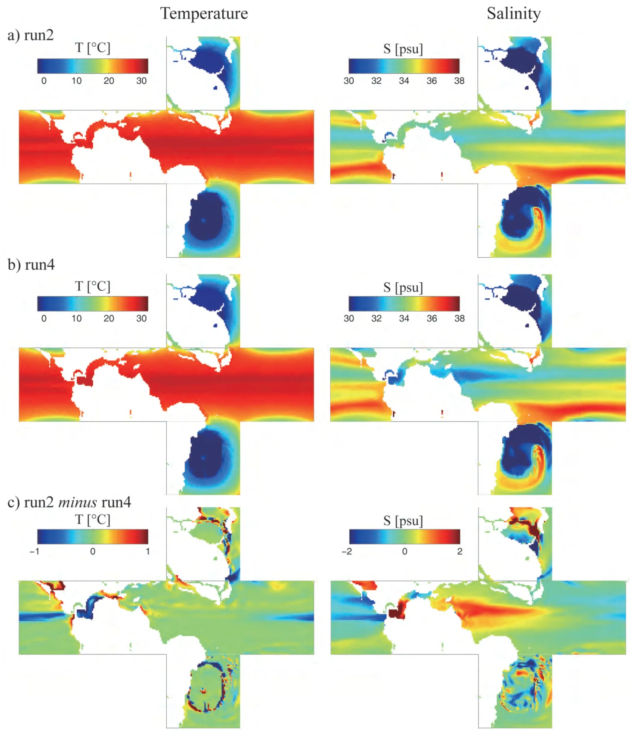
Figure 3 Final annual sea-surface temperature T (left) and sea-surface salinity S (right) for the experiment with: a) an open western boundary in the Proto-Caribbean (run2, first line); b) a closed western boundary (run4, second line); and c) anomalies between the two experiments (run2 minus run4, third line).
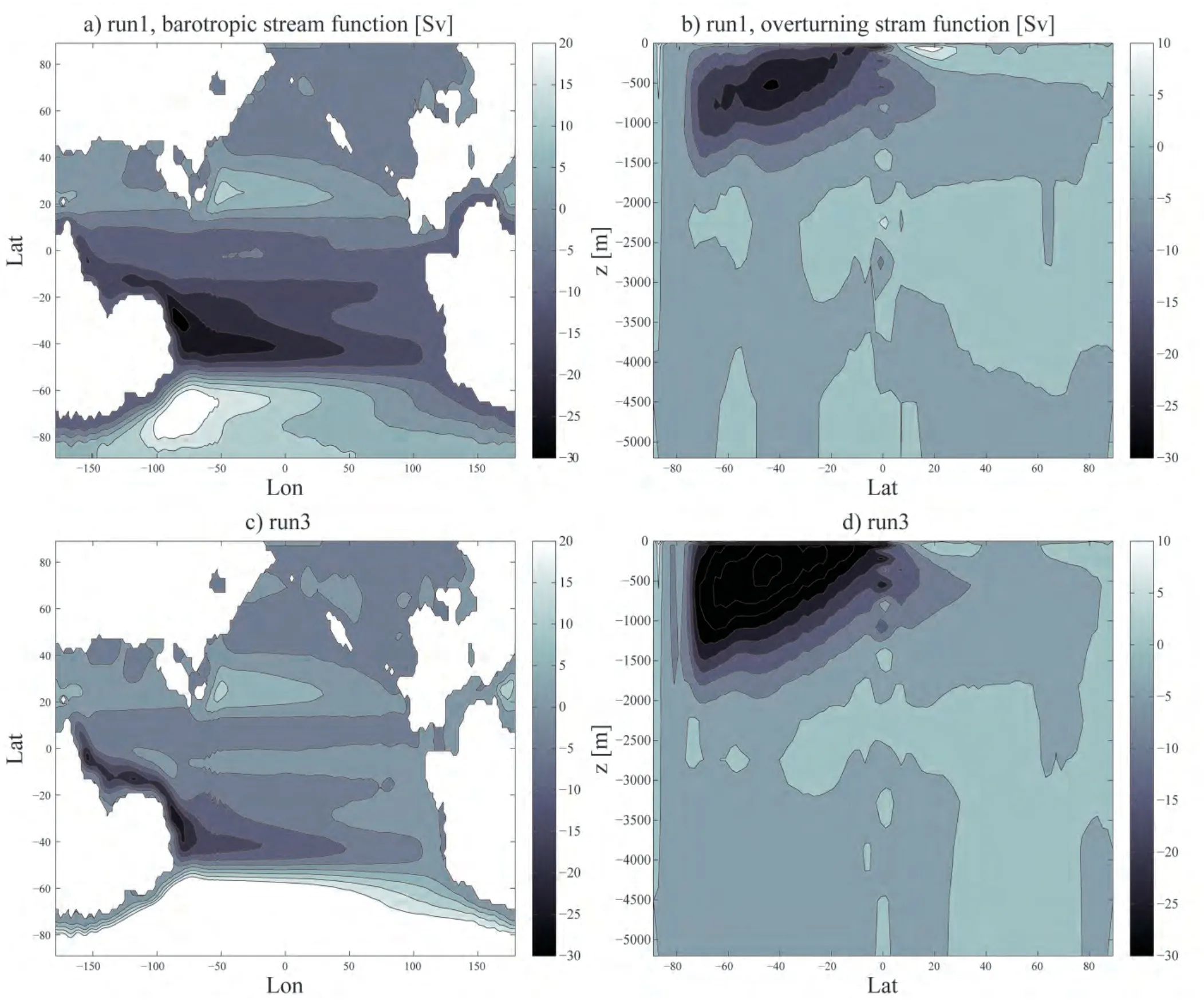
Figure 4 Barotropic stream function (left) and meridional overturning stream function (right) in Sv (1 Sv = 106 m3·s-1) for the experiments cs32 with an open western boundary in the Proto-Caribbean (run1, first line, a) and b)) and with a closed western boundary (run3, second line, c) and d)). Mean values over the last 30 model years. Clockwise circulation patterns are positive.
2) In the high resolution runs (run2 and run4, panels on the first column of Fig. 5), the intensity of the Panthalassa gyre in the northern hemisphere is modulated by the ocean bathymetry (note in particular the effects of the Proto-Pacific and of the relief elongated perpendicularly at the western boundary of Panthalassa, shown in Fig. 1). This modulation is also present but is less evident in low resolution runs.
3) The Selwyn Sea is nearly inert in all the simulations. It has a stagnant circulation, as can be seen in particular from the absence of any pattern in the meridional overturning circulation at northern high latitudes. The Arctic domain acts as a downwelling area initiating thermohaline convection in Dera and Donnadieu (2012) where the palaeogeographic reconstruction is different and consider a relatively widely open Viking corridor which significantly connects the Arctic sea to the Neo-Tethys. Such large corridor is not supported by the heuristic, physically-based synthetic topography computed on top of the plate tectonic model. In contrast, the palaeogeography used in this study (Fig. 1)suggests that rifted corridors under water had few or no connections between the Selwyn Sea on the one hand and the Neo-Tethys and/or Atlantic oceans on the other hand.
4) There is a clockwise southern current in the Austral Ocean which follows the bathymetry and becomes much less intense along the southern coast of Gondwana (in run1 and run2). The closure of the western boundary in the Proto-Caribbean has the effect of increasing the intensity of this current.
5) There is a large asymmetry of the transport in the northern and southern hemispheres, as can be observed in particular from the meridional overturning circulation. This asymmetry is a robust result which is observed in all of the simulations. This asymmetry in the meridional overturning circulation has been observed in Dera and Donnadieu (2012)for high pCO2levels.
6) In run1, a clockwise overturning cell develops at latitudes 20S-60N and depths of 2000-3000 m, which can be observed also in run2. This overturning cell becomes less intense in the closed-boundary runs (run3 and run4). In run1 and run3, a counter-clockwise cell in the southern hemisphere develops from the surface to depths of 1500-2000 m. This cell is not observed in high resolution runs(run2 and run4). This difference in the overturning circulation can explain the absence of sea-ice in the southern hemisphere in low resolution runs.
7) Changing the runoff forcing does not give any significant difference between run1 and run1a. On the contrary,if salinity forcing is changed (as in run1b, run1d and with less effect in run1c), the magnitude of the overturning cells become larger than in run1, reaching deeper waters(not shown), even if the overall patterns of the barotropic stream function and of the overturning circulation are similar to those obtained in run1 (Fig. 4, first line).
The westward current which flows in the nascent Atlantic Ocean is weak and limited to a depth of 1000 m. The volume transport at the eastern boundary of the Central Atlantic is listed in the last column of Table 3 for the different runs. The range of these values gives an idea of the theoretical uncertainty in the construction of the different surface forcings and experimental setup. All the numerical experiments agree in giving an annual-averaged volume transport of the order of 2 Sv (1 Sv = 106m3·s-1) in a western direction when the Proto-Caribbean is connected to Panthalassa. When this passage is blocked, the water transport is strongly reduced (compare run3 with run1, and run4 with run2 in Table 3). The mechanism of formation of the current in the Central Atlantic is the following: the Equatorial Current system, which is active in Panthalassa and in the central Neo-Tethys, reaches the Arabian margin and it is in part reflected as an Equatorial Counter Current.The North Equatorial Current enters the western Tethys:part enters the Central Atlantic and part is deflected to the North.
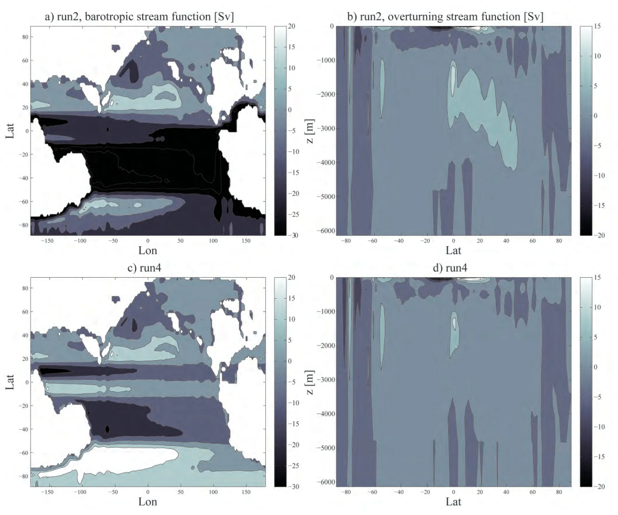
Figure 5 Barotropic stream function (left) and meridional overturning stream function (right) in Sv for the experiments cs64 with an open western boundary in the Proto-Caribbean (run2, first line, a) and b)) and with a closed western boundary (run4, second line, c) and d)).Mean values over the last 30 model years. Clockwise circulation patterns are positive.
Thus, our results indicate that the Middle Jurassic bathymetry of the Central Atlantic and Proto-Caribbean seaway only allows for a weak current (2 Sv), even if the system is open to the West (run1, run2). This is much smaller than the transport considered in idealised models (the volume transport is 600 Sv in Hotinski and Toggweiler (2003)and 1300 Sv for the aquaplanet model in Enderton and Marshall (2009), see in particular the so-called ‘EqPas’ configuration). Moreover, together with the small Equatorial passage, in the Middle Jurassic there was a gap at southern latitudes in the meridional barrier (as in the ‘Drake’ configuration in Enderton and Marshall (2009)). The meridional barrier was not uniform, since it was much wider at northern latitudes, because the land distribution in the Middle Jurassic was not symmetric with respect to the Equator(43% in the northern hemisphere and 26% in the southern hemisphere, see Fig. 1). It would be interesting to check if simplified models as those in Hotinski and Toggweiler (2003)and Enderton and Marshall (2009) can reproduce the predicted asymmetric transport of the Middle Jurassic epoch in the presence of a westward current of the order of 2 Sv in the Equatorial passage.
The shallow current enters into the Central Atlantic flowing mainly on the northern side of the basin, as can be seen in the left panel of Figure 6. The North Equatorial Current seasonally reaches the Jurassic palaeolatitudes of western Tethys (between 20°N and 40°N) and, as a consequence, the volume transport of the current through the Central Atlantic seasonally changes. If we close the Proto-Caribbean basin at its western boundary, both horizontal and vertical velocities become smaller, as results from the comparison of the two panels in Figure 6. Thus, the effect of a current flowing through the Central Atlantic would be increased upwelling, which is not consistent with the sedimentary record (Baumgartner, 2013), as discussed in section 3.
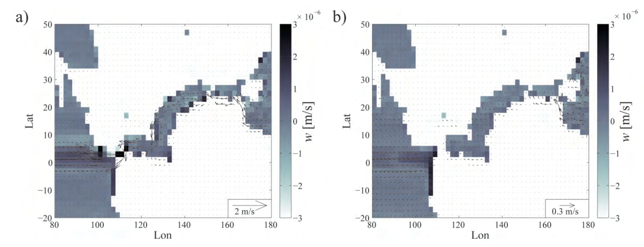
Figure 6 Current in the Central Atlantic and the Proto-Caribbean basin simulated with a) open western boundary (in run2, left); and b)with closed western boundary (in run4, right). Colors in the bar refer to the surface values of the vertical component w of the velocity in m/s (mean values over the last 30 model years). Note that the horizontal unit velocity is not the same.
6 Summary and conclusions
We analysed the ocean circulation in the Middle Jurassic(Callovian) Epoch (~165 Ma) using a coupled ocean-seaice model and a palaeo-DEM which includes detailed reconstructions of oceanic realms.
Deep-sea sediments in the Middle Jurassic Central Atlantic and Proto-Caribbean exclude models involving a vigorous equatorial trans-Pangaean current. We have designed numerical experiments for testing the existence of this trans-Pangaean passage by considering both the configurations with and without an open connection between the Proto-Caribbean and Panthalassa.
We have found that the Middle Jurassic bathymetry of the Central Atlantic and Proto-Caribbean only allows for a weak westward current of the order of 2 Sv in the upper 1000 m if the system is open at the West. The configuration with a closed western boundary to the Proto-Caribbean gives rise to reduced upwelling, in agreement with deepsea sediments which suggest that oligotrophic conditions prevailed in the Central Atlantic (Baumgartner, 2013). Another effect of closing the western boundary of the Proto-Caribbean is to increase the transport associated to barotropic gyres in the southern hemisphere and to change the surface water properties (salinity and temperature) in the Neo-Tethys and the Proto-Caribbean basin.
The bathymetry of oceanic realms produces non-negligible effects on the global ocean circulation and thus we stress the importance of using palaeo-digital elevation models with detailed reconstructions of oceanic realms for ocean simulations with horizontal spatial resolutions≤2.5°. The transport associated with the barotropic gyres and the meridional overturning circulation is asymmetric with respect to the Equator. The Selwyn Sea has a stagnant circulation since the palaeogeographic reconstruction precludes open connections between the Arctic domain and Neo-Tethys.
Sea-ice develops only in experiments with high resolutions (cs64), where a different parameterisation of smallscale processes has been included (namely, vertical mixing and viscosity). The main difference in runs with and without sea-ice formation is in the meridional overturning circulation. Numerical experiments with increased resolution or different parameterisation of small-scales processes are necessary to clarify this point.
The methods developed in the present study can be applied to other geological periods. We believe that coupling of accurate dynamical ocean models and palaeo-digital elevation models with detailed reconstructions of oceanic realms is a promising method for investigating geological periods where deep-sea sediments are not conclusive or sparse, for testing/reshaping climate hypotheses, or for quantifying the response to various climatic factors.
Improvements are expected by applying coupled atmosphere-ocean-sea-ice models. The coupled approach will allow us to take into account possible feedbacks between the atmosphere and other climate components, with the effect of reducing the uncertainty related to the forcing fields and the boundary conditions.
Acknowledgements
This work was performed in the context of the CADMOS programme. We thank Martin Beniston for useful discussions. We are very grateful to Karin Warners and Cees van Oosterhout from Shell for their support and we kindly thank Shell for the permission to use their palaeo-digital elevation model (© Shell Global Solutions International, 2013;based on the 2010 version of the UNIL plate model). We acknowledge the NOAA/OAR/ESRL PSD, Boulder, Colorado(USA) for providing the NCEP Reanalysis Derived Data at http://www.esrl.noaa.gov/psd. Maura Brunetti warmly thanks Stéphane Goyette for reading the first version of this manuscript and his precious comments.
1. Adcroft, A., Campin, J.-M., Hill, C., Marshall, J., 2004. Implementation of an Atmosphere-Ocean General Circulation Model on the Expanded Spherical Cube.Monthly Weather Re‑view, 132, 2845-2863.
2. Barron, E. J., 1981. Paleogeography as a climatic forcing factor.Geologische Rundschau, 70, 737-747.
3. Baumgartner, P. O., 2013. Mesozoic radiolarites — Accumulation as a function of sea surface fertility on Tethyan margins and in ocean basins.Sedimentology, 60, 292-318.
4. Bjerrum, C. J., Surlyk, F., Callomon, J. H., Slingerland, R. L.,2001. Numerical paleoceanographic study of the Early Jurassic Transcontinental Laurasian seaway.Paleocenography, 16,390-404.
5. Bush, A. B. G., 1997. Numerical simulation of the Cretaceous Tethys circumglobal current.Science, 275, 807-810.
6. Cecca, F., Martin Garin, B., Marchand, D., Lathuiliere, B.,Bartolini, A., 2005. Paleoclimatic control of biogeographic and sedimentary events in Tethyan and peri-Tethyan areas during the Oxfordian (Late Jurassic).Palaeogeography,Pal‑aeoclimatology,Palaeoecology, 222, 10-32.
7. Chandler, M. A., Rind, D., Ruedy, R., 1992. Pangaean during the Early Jurassic: GCM simulations and the sedimentary record of paleoclimate.GSA Bulletin, 104, 543-559.
8. Danabasoglu, G., 2004. A comparison of global ocean general circulation model solutions obtained with synchronous and accelerated integration methods.Ocean Modelling, 7, 323-341.
9. Dera, G., Donnadieu, Y., 2012. Modeling evidences for global warming, Arctic seawater freshening, and sluggish oceanic circulation during the Early Toarcian anoxic event.Paleoce‑nography, 27, PA2211.
10. Donnadieu, Y., Dromart, G., GoddéRis, Y., PucéAt, E., Brigaud, B., Dera, G., Dumas, C., Olivier, N., 2011. A mechanism for brief glacial episodes in the Mesozoic greenhouse.Pale‑oceanography, 26, PA3212.
11. Donnadieu, Y., Pierrehumbert, R., Jacob, R., Fluteau, F.,2006. Modelling the primary control of palaeogeography on Cretaceous climate.Earth and Planetary Science Letters,248, 426-437.
12. Enderton, D., Marshall, J., 2009. Explorations of Atmosphere-Ocean-ice Climates on an Aquaplanet and their Meridional Energy Transports.Journal of Atmospheric Sciences, 66,1593-1611.
13. Erba, E., 1994. Nannofossils and superplumes: The early Aptian “nannoconid crisis”.Paleoceanography, 9, 483-501.
14. Ferrari, O., Hochard, C., Stampfli, G., 2008. An alternative plate tectonic constrained model for the Paleozoic-Early Mesozoic Paleotethyan evolution of the Southeast Asia, with special attention to northern Thailand.Tectonophysics, 451,346-365.
15. Flores-Reyes, K. E., 2009. Mesozoic oceanic terranes of southern Central America — Geology, geochemistry and geodynamics. University of Lausanne, Lausanne, Ph.D. Thesis, 317 pages.
16. François, I. M., Walker, J. C. G., 1992. Modelling the Phanerozoic carbon cycle and climate: Constraints from the87Sr/86Sr isotopic ratio of seawater.American Journal of Science, 292,81-135.
17. Gent, P. R., McWilliams, J. C., 1990. Isopycnal mixing in Ocean Circulation Models.Journal of Physical Oceanography,20, 150-160.
18. Griffies, S. M., Biastoch, A., Böning, C., Bryan, F., Danabasoglu, G., Chassignet, E. P., England, M. H., Gerdes, R., Haak, H.,Hallberg, R. W., Hazeleger, W., Jungclaus, J., Large, W. G.,Madec, G., Pirani, A., Samuels, B. L., Scheinert, M., Gupta, A.S., Severijns, C. A., Simmons, H. L., Treguier, A. M., Winton,M., Yeager, S., Yin, J., 2009. Coordinated Ocean-ice Reference Experiments (COREs).Ocean Modelling, 26, 1-46.
19. Hafkenscheid, E., Wortel, R., Spakman, W., 2006. Subduction history of the Tethyan region derived from seismic tomography and tectonic reconstructions.Journal of Geophysical Re‑search, 111, B08401.
20. Hay, W. W., Migdisov, A., Balukhovsky, A. N., Wold, C. N.,Flögel, S., Söding, E., 2006. Evaporites and the salinity of the ocean during the Phanerozoic: Implications for climate,ocean circulation and life.Palaeogeography,Palaeoclimatol‑ogy,Palaeoecology, 240, 3-46.
21. Hochard, C., 2008. GIS and geodatabases application to global scale plate tectonics modeling. University of Lausanne,Lausanne, Ph.D. Thesis, 164 pages.
22. Hotinski, R. M., Toggweiler, J. R., 2003. Impact of a Tethyan circumglobal passage on ocean heat transport and “equable”climates.Paleoceanography, 18, 1007.
23. Iturralde-Vinent, M. A., 2006. Meso-Cenozoic Caribbean paleogeography: Implications for the historical biogeography of the region.International Geology Review, 48, 791-827.
24. Iturralde-Vinent, M. A., Pszczólkowski, A., 2011. Geologíadel terreno Guaniguanico. In: Iturralde-Vinent, M. A., (Ed.), Compendio de Geología de Cuba y del Caribe. Editorial CITMATEL,La Habana, Cuba.
25. Kalnay, E., Kanamitsu, M., Kistler, R., Collins, W., Deaven, D.,Gandin, L., Iredell, M., Saha, S., White, G., Woollen, J., Zhu,Y., Leetmaa, A., Reynolds, B., Chelliah, M., Ebisuzaki, W.,Higgins, W., Janowiak, J., Mo, K. C., Ro-pelewski, C., Wang,J., Jenne, R., Joseph, D., 1996. The NCEP/NCAR 40-Year Reanalysis Project.Bulletin of the American Meteorological Society, 77, 437-472.
26. Kneller, E. A., Johnson, C. A., Karner, G. D., Einhorn, J., Queffelec, T. A., 2012. Inverse methods for modeling non-rigid plate kinematics: Application to mesozoic plate reconstructions of the Central Atlantic.Computers and Geosciences, 49,217-230.
27. Labails, C., Olivet, J.-L., Aslanian, D., Roest, W. R., 2010.An alternative early opening scenario for the Central Atlantic Ocean.Earth and Planetary Science Letters, 297, 355-368.
28. Large, W. G., McWilliams, J. C., Doney, S. C., 1994. Oceanic vertical mixing: A review and a model with a nonlocal boundary layer parameterization.Reviews of Geophysics, 32, 363-404.
29. Large, W. G., Yeager, S. G., 2004. Diurnal to decadal global forcing for ocean and sea-ice models: The data sets and flux climatologies. NCAR Technical Note, NCAR, Boulder, CO.
30. Levitus, S., Boyer, T. P., 1994. World Ocean Atlas, Volume 4:Temperature. U.S. Department of Commerce, Washington, D. C.
31. Markwick, P., Valdes, P., 2004. Palaeo-digital elevation models for use as boundary conditions in coupled ocean-atmosphere GCM experiments: A Maastrichian (Late Cretaceous) example.Palaeogeography,Palaeoclimatology,Palaeoecology, 213,37-63.
32. Marshall, J., Adcroft, A., Hill, C., Perelman, L., Heisey, C.,1997a. A finite-volume, incompressible Navier Stokes model for studies of the ocean on parallel computers.Journal of Geophysical Research, 102, 5753-5766.
33. Marshall, J., Hill, C., Perelman, L., Adcroft, A., 1997b. Hydrostatic, quasi-hydrostatic, and nonhydrostatic ocean modeling.Journal of Geophysical Research, 102, 5733-5752.
34. Moix, P., Beccaletto, L., Kozur, H. W., Hochard, C., Rosselet,F., Stampfli, G. M., 2008. A new classification of the Turkish terranes and sutures and its implication for the palaeotectonic history of the region.Tectonophysics, 451, 7-39.
35. Moore, G. T., Hayashida, D. N., Ross, C. A., Jacobson, S. R.,1992. Paleoclimate of the Kimmeridgian/Tithonian (Late Jurassic) world: I. Results using a general circulation model.Pal‑aegeography,Palaeoclimatology,Palaeoecology, 93, 113-150.
36. Nardin, E., Goddéris, Y., Donnadieu, Y., Hir, G. L., Blakey,R. C., Pucéat, E., Aretz, M., 2011. Modelling the Early Paleozoic long-term climatic trend.Geological Society of America Bulletin, 123, 1181-1192.
37. Pindell, J., Maresh, W. V., Martens, U., Stanek, K., 2012. The Greater Antillean Arc: Early Cretaceous origin and proposed relationship to Central American subduction mélanges: Implications for models of Caribbean evolution.International Geology Review, 54, 131-143.
38. Pindell, J. L., Kennan, L., 2009. Tectonic evolution of the Gulf of Mexico, Caribbean and northern South America in the mantle reference frame: An update.Geological Society of London Special Publications, 328, 1-55.
39. Poulsen, C. J., Gendaszek, A. S., Jacob, R. L., 2003. Did the rifting of the Atlantic Ocean cause the Cretaceous thermal maximum?Geology, 31, 115-118.
40. Prokoph, A., Shields, G. A., Veizer, J., 2008. Compilation and time-series analysis of a marine carbonate δ18O, δ13C,87Sr/86Sr and δ34S database through Earth history.Earth Sci‑ence Reviews, 87, 113-133.
41. Rees, P. M., Ziegler, A. M., Valdes, P. J., 2000. Jurassic phytogeography and climates: New data and model comparisons.In: Huber, B. T., MacLeod, K. G., Wing, S. T., (Eds.), Warm climates in Earth history. Cambridge University Press, Cambridge, pp. 297-318.
42. Rind, D., Chandler, M., 1991. Increased ocean heat transports and warmer climate.Journal of Geophysical Research, 96,7437-7461.
43. Roscher, M., Stordal, F., Svensen, H., 2011. The effect of global warming and global cooling on the distribution of the latest Permian climate zones.Palaegeography,Palaeoclimatology,Palaeoecology, 309, 186-200.
44. Saltzman, B., 2002. Dynamical Paleoclimatology. Academic Press.
45. Sellwood, B. W., Valdes, P. J., 2006. Mesozoic climates: General circulation models and the rock record.Sedimentary Ge‑ology, 190, 269-287.
46. Sellwood, B. W., Valdes, P. J., 2008. Jurassic climates.Pro‑ceedings of the Geologists’ Association, 119, 5-17.
47. Sellwood, B. W., Valdes, P. J., Price, G. D., 2000. Geological evaluation of multiple general circulation model simulations of Late Jurassic palaeoclimate.Palaeogeography,Palaeocli‑matology,Palaeoecology, 156, 147-160.
48. Stampfli, G., Borel, G., 2002. A plate tectonic model for the Paleozoic and Mesozoic constrained by dynamic plate boundaries and restored synthetic oceanic isochrons.Earth and Plan‑etary Science Letters, 196, 17-33.
49. Stampfli, G., Borel, G., 2004. The TRANSMED transects in space and time: Constraints on the paleo-tectonic evolution of the Mediterranean domain. In: Cavazza, W., Roure, F., Spakman, W., Stampfli, G., Ziegler, P., (Eds.), The TRANSMED Atlas: The Mediterranean region from crust to mantle. Springer Verlag, Berlin.
50. Stampfli, G., Kozur, H., 2006. Europe from the Variscan to the Alpine cycles. Geological Society, London, Memoirs, 32, 57-82.
51. Stampfli, G. M., 2013. Response to the comments on “The formation of Pangea” by D.A. Ruban.Tectonophysics, 608,1445-1447.
52. Stampfli, G. M., Hochard, C., Vérard, C., Wilhem, C., von-Raumer, J., 2013. The formation of Pangea.Tectonophysics,593, 1-19.
53. Stocker, T., 2011. Introduction to Climate Modelling. Springer.
54. Valdes, P., 1993. Atmospheric General Circulation Models of the Jurassic.Royal Society of London Philosophical Transac‑tions Series B, 341, 317-326.
55. Vérard, C., Flores, K., Stampfli, G. M., 2012. Geodynamic reconstructions of the South America-Antarctica plate system.Journal of Geodynamics, 53, 43-60.
56. Vérard, C., Hochard, C., Baumgartner, P. O., Stampfli, G.,2015a. 3D palaeogeographic reconstructions of the Phanerozoic versus sea-level and Sr-ratio variations.Journal of Pal‑aeogeography, 4(1), 64-84.
57. Vérard, C., Hochard, C., Baumgartner, P. O., Stampfli, G.,2015b. Geodynamic evolution of the Earth over the Phanerozoic: Plate tectonic activity and palaeoclimate indicators.Journal of Palaeogeography, 4(2), 167-188.
58. Vérard, C., Stampfli, G. M., 2013a. Geodynamic reconstructions of the Australides — 1: Palaeozoic.Geosciences, 3,311-330.
59. Vérard, C., Stampfli, G. M., 2013b. Geodynamic reconstructions of the Australides — 2: Mesozoic-Cainozoic.Geo‑sciences, 3, 331-353.
60. vonRaumer, J., Stampfli, G., Hochard, C., Gutierrez-Marco,C., 2006. The Early Paleozoic in Iberia — A plate tectonic interpretation.Zeitschrift der Deutschen Gesellschaft für Geowissenschaften, 157, 575-584.
61. Webb, P., 2012. Mantle Circulation Models: Constraining mantle dynamics, testing plate motion history and calculating dynamic topography. School of Earth and Ocean Sciences,Cardiff University, Ph.D. Thesis, 256 pages.
62. Wilhem, C., 2010. Plate tectonics of the Altaids. University of Lausanne, Lausanne, Ph.D. Thesis, 347 pages.
63. Zhang, J., Hibler, W. D., 1997. On an efficient numerical method for modeling sea ice dynamics.Journal of Geophysi‑cal Research, 102, 8691-8702.
猜你喜欢
当代陕西(2020年15期)2021-01-07
小学生学习指导(爆笑校园)(2020年3期)2020-06-05
疯狂英语·初中天地(2018年6期)2018-11-24
青年歌声(2018年4期)2018-10-20
小天使·四年级语数英综合(2018年5期)2018-07-04
乡村地理(2018年4期)2018-03-23
娃娃乐园·3-7岁综合智能(2017年7期)2018-02-01
军营文化天地(2016年10期)2016-06-15
小天使·一年级语数英综合(2016年7期)2016-05-14
中国卫生(2015年10期)2015-11-10
 Journal of Palaeogeography2015年4期
- Journal of Palaeogeography的其它文章
- End-Triassic nonmarine biotic events
- Correction of two Upper Paleozoic stratigraphic units in the Tianshan Mountains region, Xinjiang Uygur Autonomous Region and implications on the Late Paleozoic evolution of Tianshan tectonic complex,Northwest China
- Lithofacies palaeogeography of the Carboniferous and Permian in the Qinshui Basin, Shanxi Province, China