
STABILITY OF VISCOUS SHOCK WAVES FOR THE ONE-DIMENSIONAL COMPRESSIBLE NAVIER-STOKES E QUATIONS WITH DENSITY-DEPENDENT VISCOSITY∗
2016-04-18 05:43LinHE何躏ShaojunTANG唐少君TaoWANG王涛SchoolofMathematicsandStatisticsWuhanUniversityWuhan430072China
关键词:王涛
Lin HE(何躏)Shaojun TANG(唐少君)Tao WANG(王涛)School of Mathematics and Statistics,Wuhan University,Wuhan 430072,China
STABILITY OF VISCOUS SHOCK WAVES FOR THE ONE-DIMENSIONAL COMPRESSIBLE NAVIER-STOKES E QUATIONS WITH DENSITY-DEPENDENT VISCOSITY∗
Lin HE(何躏)Shaojun TANG(唐少君)†Tao WANG(王涛)
School of Mathematics and Statistics,Wuhan University,Wuhan 430072,China
E-mail:Linhe1989@whu.edu.cn;shaojun.tang@whu.edu.cn;tao.wang@whu.edu.cn
AbstractWe study the large-time behavior toward viscous shock waves to the Cauchy problem of the one-dimensional compressible isentropic Navier-Stokes equations with densitydependent viscosity.The nonlinear stability of the viscous shock waves is shown for certain class of large initial perturbation with integral zero which can allow the initial density to have large oscillation.Our analysis relies upon the technique developed by Kanel′and the continuation argument.
Key wordsviscous shock waves;density-dependent viscosity;one-dimensional compressible Navier-Stokes equations;nonlinear stability;large density oscillation
2010 MR Subject Classi fi cation35B35;35Q35;76L05;76N15
∗Received February 3,2015;revised May 20,2015.This work was supported by“the Fundamental Research Funds for the Central Universities”.
†Corresponding author:Shaojun TANG.
1 Introduction
We consider the large time behavior of global solutions to Cauchy problem of the onedimensional compressible isentropic Navier-Stokes equations with density-dependent viscosity in Lagrangian coordinates

with prescribed initial conditions

here t>0 is the time variable,x∈R is the Lagrangian spatial variable,and v±>0,u±are given constants.The primary dependent variables are the speci fi c volume v and the velocity u.Throughout this manuscript,the pressure p and the viscosity coeffi cientµare given by

where γ>1 represents the adiabatic exponent,a>0,b>0 and κ are the gas constants.Without loss of generality,we can assume that a=b=1 in the rest of this manuscript.
Before stating the main problem studied in this manuscript,we first explain our motivation to study the one-dimensional compressible Navier-Stokes equations(1.1)satisfying relations(1.3).According to the study on the kinetic theory of dilute gases,if one derives the one-dimensional compressible Navier-Stokes equations from the Boltzmann equation with slab symmetry through the Chapman-Enskog expansion(see Chapman-Cowling[1]),one can deduce that the fi ve thermodynamical variables,i.e.,the density ρ=v−1,the temperature θ,the internal energy e,the entropy s,and the pressure p,satisfy the equations of the state of the ideal polytropic gases

for some positive constants l>1,R>0,˜b>0,cv>0 and the viscosity coeffi cientµtogether with the heat conductivity coeffi cient κ are no longer positive constants but depend on the temperature.In fact for the cuto ff inverse power force model(cf.[14]),the interacting potential between molecules is proportional to r1−swhere r denotes the distance between molecules and s>5 is a constant and in such a case,one can deduce by employing the properties of the Burnett functions that the viscosity coeffi cientµand the heat conductivity coeffi cient κ satisfy

Note that as s→+∞,the cuto ff inverse power force model is then reduced to the hard sphere model,while the Maxwell molecule model corresponds to the case of s=5.
For isentropic polytropic flows,the pressure psatisfies p=ãργfor some positive constants ã>0,γ≥1.Such a fact together with(1.4)imply

Thus for isentropic polytropic flows,one can get from(1.5)and(1.6)that the dependence of the viscosity coeffi cientµon θ can be transferred into the dependence ofµon the density as

which is nothing but(1.3)withIt is worth to pointing out that although the fact that s>5 from physical consideration implies thatto illustrate the range of the parameters γ and κ to which our argument can be applied,we will deal with the case when(1.3)hold with the constant κ being independent of γ in the rest of the paper.
The problem we want to study is on the time-asymptotically nonlinear stability of viscous shock waves for the Cauchy problem(1.1)-(1.2).Recall that a viscous shock wave of(1.1)connecting(v−,u−)and(v+,u+)is a traveling wave solution(v,u)(t,x)≡(V,U)(x−st)of(1.1)satisfying

where s is the shock speed and(vl,ul)and(vr,ur)are the given far- field states satisfying(v+,u+)∈S1S2(v−,u−),where

Under the above assumptions imposed on the far- fields(v±,u±)of the initial data,following the standard arguments in[16],we canfind a uniquesuch that(v+,u+)∈where

is the i-shock curve passing through(vl,ul).It is easy to show that the system(1.1)admits a 1-viscous shock wave(V1,U1)(x−s1t)connecting(v−,u−)with(¯v,¯u)and a 2-viscous shock wave(V2,U2)(x−s2t)connecting(¯v,¯u)with(v+,u+),and both of them are unique up to a shift,where s1=s1(v−,¯v)<0 and s2=s2(v+,¯v)>0.It is expected that the large-time behavior of global solutions of the Cauchy problem(1.1)-(1.2)is described by the superposition of the shifted 1-viscous shock wave(V1,U1)(x−s1t+α1)and the shifted 2-viscous shock wave(V2,U2)(x−s2t+α2):

where the shifts α1and α2are given by

with
Before stating our main result,we first recall some previous results closely related.For the case when the viscosity coeffi cientµ(v)is a constant,stability of viscous shock wave for small initial perturbation with“zero mass”condition was proved in Kawashima-Matsumura[8]for small-amplitude profile and in Matsumura-Nishihara[13]where the corresponding assumption imposed on the amplitude of the viscous shock profile is relaxed to the assumption that

Notice that

although for general γ>1,especially for the case when γ is sufficiently large,assumption(1.13)holds only when the strength of the viscous shock profile is sufficiently small,it does hold for any vland vrif γ→1.Later,there appeared many works treating the case when the initial perturbation is not of zero mass.In particular,the asymptotic stability for small-amplitude viscous shock wave of(1.1)and related physical systems was studied in Mascia-Zumbrun[10]and Liu-Zeng[9]with small initial perturbation.As for the asymptotic stability of viscous shock wave with large initial perturbation,it was a long-standing challenging open problem,except for the partial result obtained in[17]where viscous shock waves were shown to be time-asymptotically stable for a certain class of large initial perturbation.
For the case when the viscosity coeffi cientµ(v)is assumed to satisfy(1.3),there is a huge literature on mathematical studies of the compressible Navier-Stokes equations with densitydependent viscosity with various initial and boundary conditions.We here just mention someworks on the large-time behavior of the solutions.Jiu-Wang-Xin[5,6]proved the timeasymptotic stability of rarefaction waves to the one-dimensional compressible Navier-Stokes equations with density-dependent viscosity for general initial data which may contain the vacuum.As for the stability of viscous shock wave,Matsumura-Wang[14]showed that any viscous shock wave of the system(1.1)-(1.3)with κ≥(γ−1)/2 is asymptotically stable for small initial perturbations with“zero mass”condition.For the corresponding result with large initial perturbation,to the best of our knowledge,no result was obtained.The main purpose of this manuscript is devoted to this problem and what we want to show in this paper is that the viscous shock wave of the compressible Navier-Stokes equations(1.1)is still nonlinear stable for certain class of large initial perturbation which satisfies the“zero mass”condition but can allow the initial density to have large oscillation.
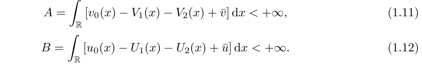
Now we turn to state our main result.To do so,we need first to introduce some notations as in the following:the strengths of the 1-viscous shock wave and the 2-viscous shock wave are denoted byrespectively.We also set δ:=|u+−u−|,and

Second,we list some assumptions on the initial data(v0,u0),the strengths of the viscous shock waves δ1,δ2,and the shifts α1,α2as follows:
(H0)there exist δ-independent constants ℓ≥0 and C0>0 such that for each x∈R,

(H1)(v+,u+)∈S1S2(v−,u−)andsuch that
(H2)the strengths of the viscous shock waves δ1,δ2,the shifts α1,α2de fined by(1.10)and the initial data(v0,u0)are assumed to satisfy
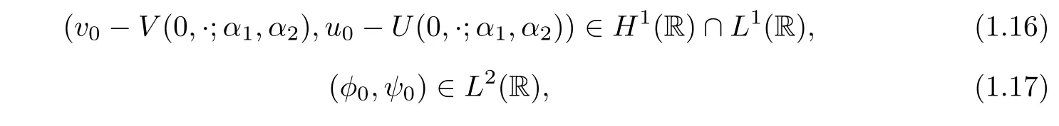
and for some positive constant C1independent of δ,

(H3)v−and v+are positive constants independent of δ.
With the above preparations in hand,we are now ready to state our main result.
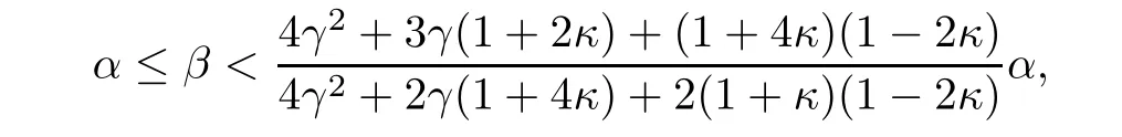
Theorem 1.1Under assumptions(H0)-(H3),we assume further that 0≤κ<12,γ>1 and

hold for some δ-independent positive constants C2,α and β.If the parameters ℓ,α and β are assumed to satisfy

then there exists a suitably small δ0>0 such that if 0<δ≤δ0,the Cauchy problem(1.1)-(1.2)has a unique solution(v,u)satisfying

and

for some positive constant C3independent of δ.Furthermore,it holds that

Remark 1.2It is easy to see that the set of the parameters α>0,β>0,ℓ≥0 which satisfy assumption(1.20)is not empty.In fact,since 0≤κ<12implies that

such that(1.20)holds.
Remark 1.3If the parameter α,β,ℓ satisfy min{2α−(γ+1)ℓ,1/2}<2(β+ℓ(1+ κ)),then for δ>0 sufficiently small,we can deduce from(1.21)that for each fixed t≥ 0,Oscv(t):=the oscillation of v(t,x),can be large in our result.We must point out,however,that the H1-norm of the initial perturbation together with the strength of the viscous shock wave are assumed to be sufficiently small in our analysis.It would be a very interesting problem to show that the viscous shock wave to the compressible Navier-Stokes equations(1.1)is nonlinear stable under general large initial perturbation or even the time-asymptotically nonlinear stable of large-amplitude viscous shock waves for a certain class of large initial perturbation like this manuscript.Note that the nonlinear stability of large-amplitude viscous shock waves to the compressible Navier-Stokes equations with constant viscosity coeffi cients under small initial perturbations is treated in[19].
Before concluding this section,we outline the main idea used in this paper.For generalγ>1,the argument employed in[8,13]relies heavily on the smallness of both δi(i=1,2)and the H2(R)-norm of the initial perturbation.One of the key points in such an argument is that,based on the a priori assumption that the H2(R)-norm of the perturbation is sufficiently small,one can deduce a uniform lower and upper positive bounds on the speci fi c volume v(t,x).With such a bound on v(t,x)in hand,one can thus deduce certain a priori H2(R)energy-type estimates on the perturbations in terms of the initial perturbation(φ0,ψ0)provided that the strengths of the viscous shock waves are suitably small.The combination of the above analysis with the standard continuation argument yields the local stability of weak viscous shock waves for the one-dimensional compressible Navier-Stokes equations with constant viscosity.
As in[3,11,15]where the global stability of rarefaction waves for the one-dimensional compressible Navier-Stokes equations with constant viscosity was investigated,the main di fficulty for deriving the global stability of viscous shock waves is to deduce the uniform lower and upper bounds on the speci fi c volume v under large initial perturbation.In this paper,we use the smallness of the strengths of viscous shock waves and the H1(R)-norm of the initial perturbation to control the possible growth of the solutions caused by the nonlinearity of the system itself,and then to derive the desired uniform lower and upper bounds on the speci fi c volume v.It is worth pointing out that the argument developed by Kanel′in[7]plays an essential role in our analysis.
The layout of this paper is as follows.After listing some notations in the rest of this section,we will state some properties of the viscous shock waves and reformulate the problem in Section 2,while Section 3 is devoted to the proof of Theorem 1.1.
NotationsThroughout this paper,c and C are used to denote various generic positive constants which are independent of δ,the strength of the viscous shock wave.We will use A≲B(B≳A)if A≤CB for some positive constant C.The notation A~B means that both A≲B and B≲A.For function spaces,Lq(Ω)(1≤q≤∞)denotes the usual Lebesgue space on Ω⊂R with norm‖·‖Lq(Ω),while Hq(Ω)denotes the usual Sobolev space in the L2sense with norm‖·‖Hq(Ω).To simplify the presentation,we use‖·‖and‖·‖qto denote‖·‖L2(R)and‖·‖Hq(R),respectively.The notation(V,U)(t,x)will be used to denote(V,U)(t,x;α1,α2)in the rest of this manuscript.
2 Preliminaries
We collect some basic properties of the viscous shock waves(Vi,Ui)(t,x)(i=1,2)and their superposition(V,U)(t,x).
We first state the existence of the viscous shock waves(Vi(x−sit),Ui(x−sit))(i=1,2)together with their decay estimates as x−sit→±∞.By using the assumption(H3),a similar proof used in[4]leads to the following lemma.We omit its proof here.
Lemma 2.1Assume that assumptions(H0)-(H3)hold,then(1.1)admits a viscous shock wave(V1,U1)(x−s2t)of the first family connecting(v−,u−)with(¯v,¯u)with speed s1and a viscous shock wave(V2,U2)(x−s2t)of the second family connecting(¯v,¯u)with(v+,u+)with speed s2,and both of them are unique up to a shift.Moreover,there exist positive constants c which depends only on v−and v+,such that,for i=1,2,

Note that(Vi,Ui)(x−sit+αi)(i=1,2)are exact solutions of the compressible Navier-Stokes equation(1.1),while their superposition(V,U)(t,x)satisfies

where

The following lemma is concerned with some estimates on g(t,x),which will play an important role in performing the energy estimates.It follows essentially from the argument in[17].Again,we omit its proof for brevity.
Lemma 2.2Under assumption(1.18),we have

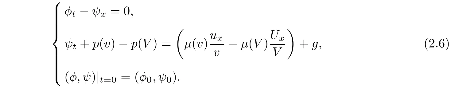
We de fi ne(φ,ψ)(t,x)by

and reformulate the original problem from(1.1)and(2.2)as
We then de fi ne the set of functions in which we find the solutions

and the local solvability of the Cauchy problem(2.6)in such a set can be stated as in the following proposition.
Proposition 2.3Let(φ0,ψ0)be in H2(R)satisfying‖(φ0,ψ0)‖2≤M0and assume that m≤V(0,x)+φ0x(x)≤M holds for each x∈R,then there exists t0>0 depending only on m,M and M0such that(2.6)has a unique solution(φ,ψ)(t,x)∈Xm/2,2M(0,t0)which satisfies for each 0≤t≤t0that

3 Proof of Theorem 1.1
In this section we first deduce some a priori estimates on the solution(φ,ψ)∈X1/m,M(0,T)to the problem(2.6),and then prove Theorem 1.1 by using the continuation argument.We willuse c and C to denote some generic positive constants independent of T,m,M and δ.Besides,we will often use the notation(v,u)=(V+φx,U+ψx),though the unknown functions are φ and ψ.Moreover,we denote here Nψ(T):=sup[0,T]‖ψ(t)‖L∝,or by Nψfor simplicity.Without loss of generality,we can assume that m≥1 and M≥1.
Our first lemma is concerned with the basic energy estimate,which is stated in the following lemma.
Lemma 3.1Under the assumptions in Theorem 1.1,there exists a sufficiently small positive constant δ1independent of δ such that if 0<δ≤δ1,then it holds for each 0≤t≤T that

where

ProofFirst,(2.6)2(second equation of(2.6))can be rewritten as

Multiply(2.6)1by φ and(3.3)by−p′(V)−1ψ to find

Since v−and v+are independent of δ and δ is assumed to be sufficiently small,we can deduce that V(t,x)can be bounded from both below and above by some positive constants independent of δ.Integrating the above identity with respect to t and x over[0,t]×R yields

Straightforward calculation leads to

Noting that Cδ2≥−Vt=−Ux>0 and using Cauchy’s and Hölder’s inequalities,we derive from(3.5)and(2.4)that for each∈>0,

Estimate(3.1)can be proved by substituting the above estimates on Ij(j=1,···,5)into(3.4)and employing the Gronwall inequality.This completes the proof of Lemma 3.1.
Lemma 3.2Under the assumptions in Theorem 1.1,if δ is suitably small,then it holds for each 0≤t≤T that

where Φ0=Φ|t=0,and

ProofMultiplying∂x(2.6)1by p(V)−p(v)and∂x(2.6)2by ψx,we obtain the following identity

Integrating this last identity over[0,t]×R yields

Since
we apply Cauchy’s inequality to I6to find

If we apply Hölder’s inequality to I7and use(2.4),we can deduce

Plugging(3.10),(3.11)and(3.5)into(3.9)and noting that

we have

which combined with(3.1)gives(3.6).The proof of the lemma is completed.
We next make the estimate on the last term of(3.6),which is stated in the following lemma.
Lemma 3.3Under the assumptions in Theorem 1.1,a δ-independent positive constant δ2exists such that if

then we have for each 0≤t≤T that

and

ProofMultiplying(2.6)2with φximplies

where we have used the fact that

Integrating(3.16)over[0,t]×R,we have from Cauchy’s and Hölder’s inequalities that

which combined with(2.4)and(3.6)implies

Noting the simple fact that

we can prove(3.14)-(3.15)and complete the proof of the lemma.
To deduce a lower bound and an upper bound on v(t,x),as in[12],we set˜v:=v/V and make the estimate onin the following lemma.
Lemma 3.4Under the assumptions in Theorem 1.1,if δ is suitably small such that(3.13)holds,then it follows that

ProofSince

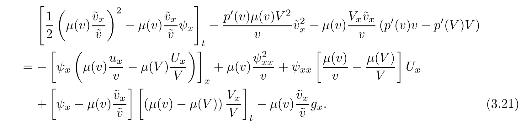
we differentiate(2.6)2and have


which combined with(3.19)and the identity

implies
For each∈>0,


Estimates(3.5)and(2.1)give

Apply(2.1)to infer

Then we apply Cauchy’s inequality and(3.24)to have
and


Integrating(3.21)over[0,t]×R and using(3.22)-(3.26),(3.14)-(3.15),and(3.13),we can obtain(3.18)by employing Gronwall’s inequality and(2.4).This completes the proof of the lemma.
The following lemma concerns the positive lower and upper bounds on v in terms of the initial perturbation.
Lemma 3.5Under the assumptions in Theorem 1.1,if we assume that(3.13)holds,then we have for each(t,x)∈[0,T]×R that

with

ProofRewrite Φ(v,V)as

and note that

In order to apply Kanel′s method[7],we constructas

From the constitutive relations(1.3),we have
which implies that


holds for some uniform constant C>0.
On the other hand,we have

For the estimates for the second order derivatives of(φ,ψ).since

we have from Lemmas 3.3-3.5 that

As for the estimate on‖ψxx(t)‖,we multiply∂x(2.6)2by ψxxx,integrate the resulting identity over[0,t]×R,and use the Sobolev’s,Young’s and Gronwall’s inequalities to discover

which combined with(3.32)yields the following lemma.
Lemma 3.6If δ is suitably small such that(3.13)holds,then we have for each 0≤t≤T that


Hence,if(1.19)and(1.20)hold,then we have for 0<δ<1,According to Proposition 2.3,there is a positive constant t1,which depends only on δ and ‖(φ0,ψ0)‖2,such that the Cauchy problem(2.6)admits a unique solution(φ(t,x),ψ(t,x))∈Xm0,M0(0,t1)with m0=2−1C−11δℓand M0=2C1(1+δ−ℓ),which satisfies(2.7)for each 0≤t≤t1.Hence we have from(1.19)and Sobolev’s inequality that

Consequently,

Thus if(1.20)1holds,we can choose a sufficiently small constant δ1<1 such that if 0<δ≤δ1,the assumptions imposed in Lemmas 3.1-3.6 hold with T=t1,m=m−10and M=M0.Thus we have from(3.27)that for each 0≤t≤t1,

From(3.15),we can have for each 0≤t≤t1that

Next if we take(φ(t1,x),ψ(t1,x))as the initial data,we can deduce by employing Proposition 2.3 again that the unique local solution(φ(t,x),ψ(t,x))constructed above can be extended to the time internal[0,t1+t2]and satisfies

and

for each t1≤t≤t1+t2.Thus,

Set

Then one can easily deduce that if the parameters α>0,β and ℓ satisfy(1.20)3,then there exists a sufficiently small δ2>0 such that if 0<δ≤δ2,the assumptions listed in Lemmas 3.1-3.6 are satis fied with T=t1+t2,m=m−11and M=M1.Consequently,(3.35),(3.36)and(3.34)hold for each 0≤t≤t1+t2.If we take(φ(t1+t2,x),ψ(t1+t2,x))as the initial data and employ Proposition 2.3 again,we can then extend the above solution(φ(t,x),ψ(t,x))to the time step t=t1+2t2.Repeating the above procedure,we thus extend(φ(t,x),ψ(t,x))step by step to the unique global solution and(3.35),(3.36)and(3.34)hold for all t≥0.The proof of Theorem 1.1 is completed.
References
[1]Chapman S,Cowling T.The Mathematical Theory of Non-uniform Gases.3rd ed.London:Cambrige University Press,1970
[2]Chen Z Z,Xiao Q H.Nonlinear stability of planar shock profiles for the generalized KdV-Burgers equation in several dimensions.Acta Math Sci,2013,33B(6):1531-1550
[3]Duan R,Liu H X,Zhao H J.Nonlinear stability of rarefaction waves for the compressible Navier-Stokes equations with large initial perturbation.Trans Amer Math Soc,2009,361(1):453-493
[4]Huang F M,Matsumura A.Stability of a composite wave of two viscous shock waves for the full compressible Navier-Stokes equation.Comm Math Phys,2009,289(3):841-861
[5]Jiu Q S,Wang Y,Xin Z P.Vacuum behaviors around rarefaction waves to 1D compressible Navier-Stokes equations with density-dependent viscosity.SIAM J Math Anal,2013,45(5):3194-3228
[6]Jiu Q S,Wang Y,Xin Z P.Stability of rarefaction waves to the 1D compressible Navier-Stokes equations with density-dependent viscosity.Comm Partial Di ff erential Equations,2011,36(4):602-634
[7]Kanel′J.A model system of equations for the one-dimensional motion of a gas.Di ff erential Equations,1968,4:374-380
[8]Kawashima S,Matsumura A.Asymptotic stability of traveling wave solutions of systems for one-dimensional gas motion.Comm Math Phys,1985,101(1):97-127
[9]Liu T P,Zeng Y N.Shock waves in conservation laws with physical viscosity.Mem Amer Math Soc,2014,234(1105):viii+168
[10]Mascia C,Zumbrun K.Stability of small-amplitude shock profiles of symmetric hyperbolic-parabolic systems.Comm Pure Appl Math,2004,57(7):841-876
[11]Matsumura A,Nishihara K.Global asymptotics toward the rarefaction wave for solutions of viscous psystem with boundary effect.Quart Appl Math,2000,58(1):69-83
[12]Matsumura A,Nishihara K.Global stability of the rarefaction wave of a one-dimensional model system for compressible viscous gas.Comm Math Phys,1992,144(2):325-335
[13]Matsumura A,Nishihara K.On the stability of travelling wave solutions of a one-dimensional model system for compressible viscous gas.Japan J Appl Math,1985,2(1):17-25
[14]Matsumura A,Wang Y.Asymptotic stability of viscous shock wave for a one-dimensional isentropic model of viscous gas with density dependent viscosity.Methods Appl Anal,2010,17(4):279-290
[15]Nishihara K,Yang T,Zhao H J.Nonlinear stability of strong rarefaction waves for compressible Navier-Stokes equations.SIAM J Math Anal,2004,35(6):1561-1593
[16]Smoller J.Shock Waves and Reaction-Di ff usion Equations.Grundlehren der Mathematischen Wissenschaften 285.[Fundamental Principles of Mathematical Sciences].2nd ed.New York:Springer-Verlag,1994
[17]Wang T,Zhao H J,Zou Q Y.One-dimensional compressible Navier-Stokes equations with large density oscillation.Kinet Relat Models,2013,6(3):649-670
[18]Xiao Q H,Zhao H J.Nonlinear stability of generalized Benjamin-Bona-Mahony-Burgers shock profiles in several dimensions.J Math Anal Appl,2013,406(1):165-187
[19]Zumbrun K.Stability of large-amplitude shock waves of compressible Navier-Stokes equations.With an appendix by Helge Kristian Jenssen and Gregory Lyng//Handbook of Mathematical Fluid Dynamics,Vol III.Amsterdam:North-Holland,2004:311-533
猜你喜欢
Chinese Physics B(2022年11期)2022-11-21
中国动物保健(2022年2期)2022-05-05
理科爱好者(教育教学版)(2022年2期)2022-05-05
三悦文摘·教育学刊(2022年7期)2022-04-27
Plasma Science and Technology(2022年2期)2022-03-10
大众文艺(2020年23期)2021-01-04
大众文艺(2020年22期)2020-12-13
美与时代·美术学刊(2018年7期)2018-11-10
艺术家(2018年12期)2018-03-18
 Acta Mathematica Scientia(English Series)2016年1期
- Acta Mathematica Scientia(English Series)的其它文章
- SOME STABILITY RESULTS FOR TIMOSHENKO SYSTEMS WITH COOPERATIVE FRICTIONAL AND INFINITE-MEMORY DAMPINGS IN THE DISPLACEMENT∗
- STABILITY ANALYSIS OF A COMPUTER VIRUS PROPAGATION MODEL WITH ANTIDOTE IN VULNERABLE SYSTEM∗
- STABILITY OF A PREDATOR-PREY SYSTEM WITH PREY TAXIS IN A GENERAL CLASS OF FUNCTIONAL RESPONSES∗
- NONSMOOTH CRITICAL POINT THEOREMS AND ITS APPLICATIONS TO QUASILINEAR SCHRÖDINGER EQUATIONS∗
- NORMAL FAMILIES OF MEROMORPHIC FUNCTIONS WITH SHARED VALUES∗
- EDELSTEIN-SUZUKI-TYPE RESULTS FOR SELF-MAPPINGS IN VARIOUS ABSTRACT SPACES WITH APPLICATION TO FUNCTIONAL EQUATIONS∗