
POSITIVE STEADY STATES AND DYNAMICS FOR A DIFFUSIVE PREDATOR-PREY SYSTEM WITH A DEGENERACY∗
2016-09-26 03:45LuYANG杨璐
Lu YANG(杨璐)
School of Mathematics and Statistics,Lanzhou University,Lanzhou 730000,China
Key Laboratory of Applied Mathematics and Complex Systems,Gansu 730000,China
Yimin ZHANG(张贻民)
Wuhan Institute of Physics and Mathematics,Chinese Academy of Sciences,Wuhan 430071,China
E-mail∶zhangyimin@wipm.ac.cn
POSITIVE STEADY STATES AND DYNAMICS FOR A DIFFUSIVE PREDATOR-PREY SYSTEM WITH A DEGENERACY∗
Lu YANG(杨璐)
School of Mathematics and Statistics,Lanzhou University,Lanzhou 730000,China
Key Laboratory of Applied Mathematics and Complex Systems,Gansu 730000,China
Yimin ZHANG(张贻民)
Wuhan Institute of Physics and Mathematics,Chinese Academy of Sciences,Wuhan 430071,China
E-mail∶zhangyimin@wipm.ac.cn
In this article,we consider positive steady state solutions and dynamics for a spatially heterogeneous predator-prey system with modified Leslie-Gower and Holling-Type II schemes.The heterogeneity here is created by the degeneracy of the intra-specific pressures for the prey.By the bifurcation method,the degree theory,and a priori estimates,we discuss the existence and multiplicity of positive steady states.Moreover,by the comparison argument,we also discuss the dynamical behavior for the diffusive predator-prey system.
Predator-prey system;steady state solution;dynamical behavior
2010 MR Subject Classification35J20;35J60
1 Introduction
In this article,we are concerned with the following predator-prey model,
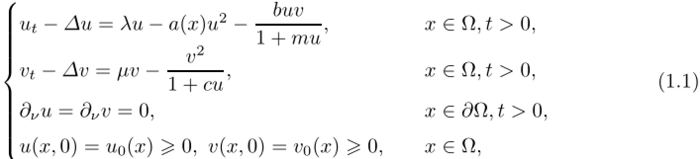
here λ,µ,b,c,m are constants,all positive exceptµ,which may take negative values;ν is the outward unit normal vector on∂Ω and∂ν=∂/∂ν;a(x),u0(x)and v0(x)are nonnegative continuous functions on a bounded smooth domain Ω⊂Rn.Moreover,there exists a subregionΩ0such thaand

We assume that Ω0is an open and connected subset of Ω,and it has C2boundary∂Ω0.
In recent years,there have been extensive attentions for the following diffusive predatorprey model with modified Leslie-Gower and Holling-Type II schemes:
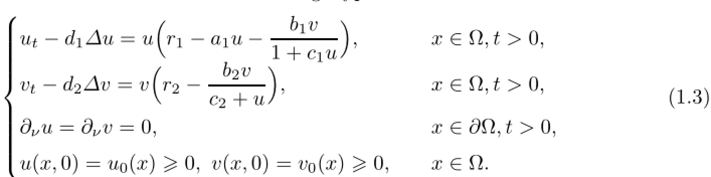
The homogeneous Neumann boundary condition means that model(1.3)is self-contained and has no population flux across the boundary∂Ω.All parameters appearing in model(1.3)are assumed to be positive constants.The constants d1and d2are the diffusion coefficient corresponding to u and v,and the initial data u0(x)and v0(x)are continuous functions.As the variables u and v account for the densities of prey and predator,they are required to be non-negative.It is clear that(1.3)has a unique global solution(u,v).In addition,if u06≡0,v06≡0,the solution is positive,that is,u(x,t)>0,v(x,t)>0 on Ω for any t>0.For the more detailed biological background of the model,see[1]and references therein.The corresponding ODE version was discussed in[1],where the authors obtained some results for the global stability of the interior equilibrium.In[8,14],Du et al considered(1.3)with c2=0 and obtained many results for non-constant positive steady states in the so-called heterogeneous environment.In contrast,[25]was mainly devoted to the studies of effects of diffusion coefficients on the positive non-constant solutions to(1.3)when c2=0.In[3],Chen and Wang mainly investigated the large-time behavior of solutions and the existence and non-existence of non-constant positive steady states for the non-dimensionalized form of(1.3)with positive constant coefficients.
The reaction-diffusion system with spatially homogeneous coefficients have been widely and extensively studied since the 1970s.While some interesting articles investigating the heterogeneous effect of environment have appeared in recent years.Dancer and Du[5]and Du et al[8,10-14]studied the effects of the heterogeneous environment caused by the protection zone or the degeneracy of some intra-specific pressures.The effects of spatially heterogeneous birth rates was shown by Dockery et al[6]and Hutson et al[15-18]for some diffusive competition models.
More recently,in[27]Wang and Li consider the following predator-prey model with crossdiffusion and protection for the prey:

where Ω⊂Rnis a bounded domain,Ω0is a smooth domain satisfying Ω0⊂Ω;ρ(x)=1 and b1(x)=b>0 in ΩΩ0,whereas ρ(x)=b1(x)=0 in Ω0.The nonlinear diffusion term τ∆[ρ(x)vu]is usually referred to as the cross-diffusion term.Such domain Ω0ia called as protection zone,which was first proposed by Du and Shi in[11].In[27],they mainly investigatedthe effects of cross-diffusion and protection zone on positive steady states of(1.4).For more works on the predator-prey system with cross-diffusion,see[19-24,28]and references therein.
In[5],Dancer and Du first studied the effect of the degeneracy of some intra-specific pressures on the diffusive Lotka-Volterra model and obtained some interesting results.Subsequently,in[13]Du and Shi investigated the Allee effect and bistability in the diffusive predator-prey model with the degeneracy of some intra-specific pressures and Holling-Type II functional responses.Motivated by some ideas in these works,we will deal with the existence and multiplicity of positive steady states and dynamical behavior of(1.1)in the spatially heterogeneous environment caused by the degeneracy of some intra-specific pressures for the prey.Finally,we point out that the main difference of(1.1)and(1.3)is the degeneracy and non-degeneracy of the coefficients for the item u2in the equation of the prey.In particular,the case of degeneracy for(1.1)does include the case of non-degeneracy(that is,Ω0=Φ),especially the case of the positive constant coefficients.To the best of our knowledge,even under the case of non-degeneracy our results are also new.
The rest of this article is organized as follows.In Section 2,we give some preliminary results including the results of the linear eigenvalue problems with a weight function and the scalar elliptic equation with a degeneracy.In Section 3,we discuss the existence of positive steady state solutions to(1.1)by the bifurcation analysis and degree theory.In Section 4,we investigate the dynamical behavior of(1.1)by the comparison argument.
2 Some Preliminaries
Linear eigenvalue problems will play important roles in our analysis.We define λD1(φ,O)and λN1(φ,O)to be the principal eigenvalues of−∆+φ over the region O,with Dirichlet or Neumann boundary conditions respectively.If the region O is omitted in the notation,then we understand that O=Ω.If the potential function φ is omitted,then we understand that φ=0. We recall some well-known properties of λD1(φ,O)and λN1(φ,O):

When describing the bifurcation properties of steady state solutions to(1.1),we will need the knowledge of the scalar equation:

Lemma 2.1([7,9])Problem(2.1)has a unique positive solution uλ(x)when 0<λ<λD1(Ω0),and it has no positive solution when λ≥λD1(Ω0).
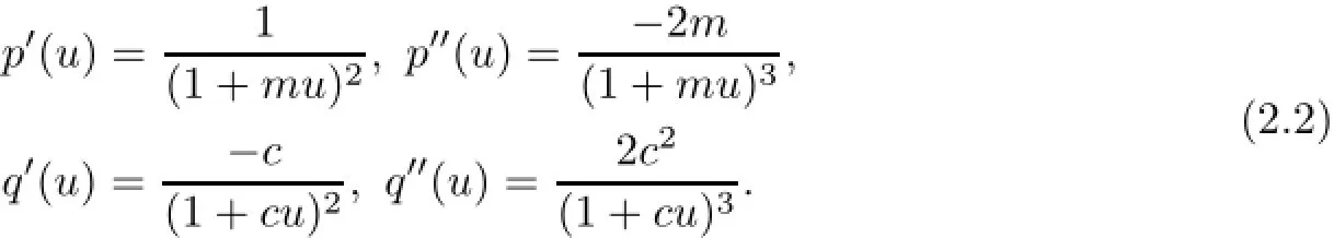
In the following analysis,we will fix 0<λ<λD1(Ω0),and we will use the predator growth rateµas a bifurcation parameter.We also fix the parameters b,m>0 unless otherwise stated. For simplicity of the notations,we will write p(u)=u/(1+mu),q(u)=1/(1+cu).It is easy to see that
3 Steady State Solutions
In this section,we will consider the structure of the set of nonnegative steady state solutions to(1.1)by the local bifurcation theory and global bifurcation theory.
3.1Steady state solutions:bifurcation analysis
For anyµ>0,(1.1)has two semi-trivial steady state solutions:(uλ,0)and(0,µ).So,we have two curves of these steady state solutions in the space of(µ,u,v):

By the strong maximum principle,any nonnegative steady state solution(u,v)of(1.1)is either(0,0),or a semi-trivial solution,or a positive solution.
From standard local bifurcation analysis,there is a bifurcation pointµ1=0 such that a smooth curve Γ′1of positive steady state solutions to(1.1)bifurcates from Γuat(µ,u,v)=(µ1,uλ,0).Similarly,there is another bifurcation pointµ2=λb−1such that a smooth curve of positive steady state solutionsto(1.1)bifurcates from Γvat(µ,u,v)=(µ2,0,µ2).From global bifurcation theory,each ofandis contained in a global branch of positive steady state solutions to(1.1).We call these branchesandrespectively.Then,as in[2]either Γ1and Γ2are both unbounded,or Γ1=Γ2.To show that the latter is the case,we prove the following proposition:
Proposition 3.1Suppose that 0<λ<and that(u,v)is a positive steady state solution of(1.1).Then,the following hold:
(i)The parameterµmust satisfy

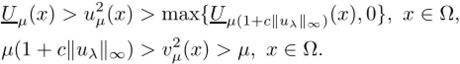
(ii)0<u(x)<uλ(x),andµ<v(x)<µ(1+c‖uλ‖∝),
where uλis the unique positive solution of(2.1).
ProofConclusion(ii)is a simple consequence of a standard comparison argument.
For conclusion(i),from conclusion(ii)and the first equation of(1.1),we have
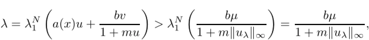
which impliesµ<λb−1(1+m‖uλ‖∝).
From Proposition 3.1,we conclude that(1.1)has no unbounded branches of positive steady state solutions when 0<λ<is fixed.Thus,the two local branches must be connected. To get a more precise local picture of Γ≡Γ1≡Γ2,we give more details on the bifurcation analysis by the bifurcation result of Crandall-Rabinowitz[4].
Theorem 3.2Suppose that 0<λ<Then,there exists a continuum Γ of positive steady state solutions of(1.1)satisfying


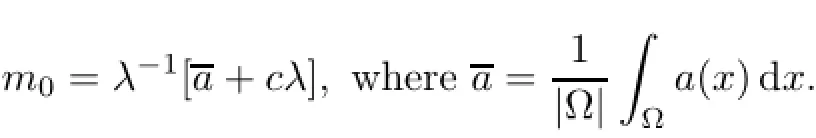
whereand Γ contains Γ1and Γ2.Moreover,the bifurcation of Γ1at(0,uλ,0)is supercritical(0)>0),and the bifurcation of Γ2at(λb−1,0,λb−1)is supercritical(0)>0)if m>m0and it is subcritical(0)<0)if 0≤m<m0,where m0is defined as
ProofFirst,we use a change of variables v=µ+w(so that(u,w)=(0,0)is the trivial steady state solution).For p>1,let X={u∈W2,p(Ω):∂νu=0},and let Y=Lp(Ω).Define F:R×X×X→Y×Y as
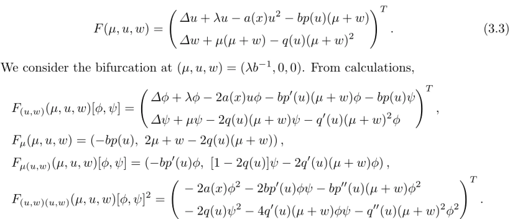
At(µ,u,w)=(λb−1,0,0),it is easy to verify that the kernel N(F(u,w)(λb−1,0,0))=span{(1,cµ)},the range R(F(u,w)(λb−1,0,0))={(f,g)∈Y2:RΩf(x)dx=0},and Fµ(u,w)(λb−1,0,0)[1,cµ]=[−b,cµ]6∈R(F(u,w)(λb−1,0,0)).Thus,we can apply the result of[4]to conclude that the set of positive steady state solutions to(1.1)near(λb−1,0,µ)is a smooth curve

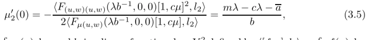
such thatµ2(0)=λb−1,u2(s)=s+o(s),and w2(s)=cs+o(s).Moreover,µ′2(0)can be calculated(see,for example,[26]):
where a=|Ω|−1Ωa(x)dx,and l2is a linear functional on Y2defined by〈[f,g],l2〉=
Ωf(x)dx. By(3.5),we know thatµ′2(0)>0 if m>m0and thatµ′2(0)<0 if 0≤m<m0.
We can do a similar analysis at(µ1,uλ,0),whereµ1=0.We change the variables w= uλ−u.Define G:R×X×X→Y×Y as

Then,


At(µ,w,v)=(µ1,0,0),it is easy to verify that the kernel N(G(w,v)(µ1,0,0))=span{(ϕ1,1)},where ϕ1satisfies

The range
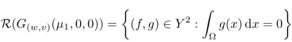
and

Thus,we can apply the result of[4]to conclude that the set of positive steady state solutions to(1.1)near(µ1,0,0)is a smooth curve

withµ1(0)=0,w1(s)=sϕ1(x)+o(s),and v1(s)=s+o(s).Moreover,
where l1is a linear functional on Y2defined by〈[f,g],l1〉=RΩg(x)dx.
By virtue of Theorem 3.2,we immediately have the following conclusion.
Corollary 3.3Suppose that 0<λ<Then,problem(1.1)has at least one positive steady state solution for allµ∈(0,λb−1).
Remark 3.4Corollary 3.3 can also be proved by a continuation and topological degree argument.For the details,see the proof of[8],Theorem 3.4].
3.2Steady state solutions:multiplicity
Notice that in(1.1),if c=0,then the steady state solution of the second equation is v(x)≡0 or v(x)≡µ.Thus,any positive steady state solution of(1.1)(u,v)satisfies v=µ(µ≥0)and u is a solution of the following equation:


whereˆµ∗=sup{µ>0:(3.10)has a positive solution}≥λb−1.Moreover,Σ satisfies the following:
(i)Near(µ,u)=(λb−1,0),Σ is a curve.
(ii)Whenµ≤0,(3.10)has a unique positive solutionand:µ≤0}is a smooth curve.
(iii)Forµ∈(−∞,ˆµ∗),(3.10)has a maximal positive solutionand(x)is strictly decreasing with respect toµ.
(iv)Forµ∈(−∞,λb−1),(3.10)has a minimal positive solutionis strictly decreasing with respect roµ.
(v)Ifˆµ∗>λb−1,then(3.10)has a maximal positive solution forµ=ˆµ∗and has at least two positive solutions for
(vi)Ifˆµ∗>and 0<m<m0,then there existsˆµ∗∈(0,λb−1)such that(3.10) has at least three positive solutions forµ∈)andMoreover=0 uniformly for x∈Ω. All these solutions mentioned above can be chosen from the unbounded continuum Σ.
On the basis of the results above,we can obtain a rather clear description of the set of positive steady state solutions of(1.1)for small c>0.
Theorem 3.6Suppose that 0<λ<)and that b,c,m>0 are fixed.Letˆµ∗and ˆµ∗be the critical points defined as in Lemma 3.5.Then,the following hold:
(i)Define

and
µ∗=inf{µ>0:(1.1)has a positive steady state solution(u,v),and u
(ii)Forµ∈(0,ˆµ∗(1+c‖uλ‖∝)−1],(1.1)has a positive steady state solutionsatisfying

(iii)Ifˆµ∗(1+c‖uλ‖∝)<λb−1,then forµ∈[ˆµ∗(1+c‖uλ‖∝),λb−1),(1.1)has a positive steady state solution()satisfying
(iv)Ifˆµ∗>λb−1(1+c‖uλ‖∝),then(1.1)has at least two positive steady state solutions for λb−1<µ≤ˆµ∗(1+c‖uλ‖∝)−1.
(v)Ifˆµ∗>λb−1(1+c‖uλ‖∝)andˆµ∗<λb−1(1+c‖uλ‖∝)−1,then(1.1)has at least three positive steady state solutions forˆµ∗(1+c‖uλ‖∝)<µ<λb−1. All these solutions above can be chosen from the continuum Γ.
ProofIf(1.1)has a positive steady state solution(u,v),then from Proposition 3.1,µ<v<µ(1+c‖uλ‖∝).Thus,u is a subsolution of(3.10),and uλ>u is always a supersolution of(3.10),so(3.10)has a positive solution for thisµ.Hence,µ∗≤ˆµ∗.Similarly,ˆµ∗≤µ∗.The proofs ofˆµ∗(1+c‖uλ‖∝)−1≤µ∗andµ∗≤ˆµ∗(1+c‖uλ‖∝)are apparent from Part(ii)and(iii)to be proved below.
We will show the existence of)forµ∈(0,ˆµ∗(1+c‖uλ‖∝)−1].Let E=C(Ω),and let P={u∈E:u(x)≥0,x∈Ω}.Define an order interval in P2=P×P:

where[u1,u2]={u∈E:u1(x)≤u(x)≤u2(x)}.We define an operator
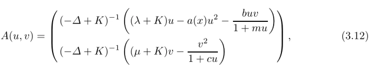
where(u,v)∈J1,and K is a positive constant.It is seen that a fixed point of A is a steady state solution of(1.1).We claim that when K is large enough,then A(u,v)∈J1for each(u,v)∈J1.Let(u,v)∈J1,and let A(u,v)=(u1,v1).We choose K large enough so that fK(x,u,v)=(λ+K)u−a(x)u2−buv/(1+mu)is strictly increasing in u and gK(u,v)=(µ+K)v−v2/(1+cu)is strictly increasing in v,for any u∈[minxand v∈[µ,µ(1+c‖uλ‖∝)].Then,
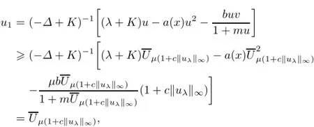
and similarly,
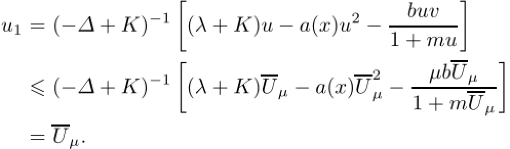
On the other hand,


because the minimum of f1(v)=(µ+K)v−v2on[µ,µ(1+c‖uλ‖∝)]is achieved at v=µ;andbecause the maximum of f2(v)=(µ+K)v−v2/(1+c‖uλ‖∝)on[µ,µ(1+c‖uλ‖∝)]is achieved at v=µ(1+c‖uλ‖∝).Therefore,(u1,v1)=A(u,v)∈J1.As A is a compact operator from the convex set J1to J1,A has a fixed point in J1by the Schauder point theorem.This completes the proof of Part(ii),and the proof of Part(iii)is similar.
We define a subset of R×P2for each~µ∈(0,ˆµ∗(1+c‖uλ‖∝)−1]:

We notice that{µ}×J1⊂J~µifµ∈(0,ˆµ∗(1+c‖uλ‖∝)−1]andµ≤~µ.Thus,(µ)∈Jµfor 0<µ≤~µ.If(µ,u,v)∈∂J~µandµ∈(0,~µ),then from the above calculation of(u1,v1)= A(u,v),we can see that either(µ,u1,v1)=(µ,0)or(µ,u1,v1)∈int(J~µ).Hence,(µ,u,v)cannot be a positive fixed point of A.
Let Γ be the continuum of positive steady state solutions of(1.1)obtained in Theorem 3.2. Then,Γ∪J~µ6=Φ because the bifurcation at(0,0)is supercritical.From the arguments above,if(µ,u,v)∈Γ∩∂J~µ,then eitherµ=0 orµ=~µ.The latter case must happen because(1.1)has no positive steady state solution whenµ=0.From the connectedness of Γ,we see thatTherefore,has a component connecting(λb−1,0,λb−1)to a solution(µ,u,v)∈,and by the above discussion,we must haveµ=ˆµ∗(1+c‖uλ‖∝)−1.Therefore,(1.1)has at least one positive steady state solution for λb−1<µ≤ˆµ∗(1+c‖uλ‖∝)−1,which is onThis proves Part(iv).
For Part(v),we use the minimal positive steady state solutions to define a set J similar toand then show thatcontains a positive solution in J and another one outside J.As the arguments are analogous,we omit the details.
4 Dynamical Behavior
First,we recall the dynamics of the auxiliary equation:
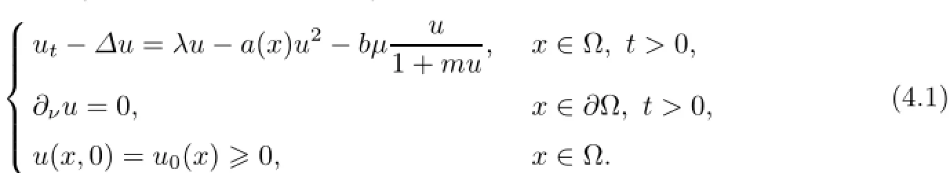
Lemma 4.1([13])Suppose that 0<λ<and that b,c,m>0 are fixed.Then,all solutions u(x,t)of(4.1)are globally bounded,and the following hold:
(ii)Ifµ>ˆµ∗,then 0 is globally asymptotically stable.
(iii)If 0<µ<λb−1,then for any u0
(iv)If 0<µ≤ˆµ∗,then for any u0,thenu(x,t)=if u0(x)≥(x),then

where Vµ,1(x)is the unique positive solution of

with U=Uˆµ∗.
(v)Ifˆµ∗<λb−1,ˆµ∗<µ<λb−1,and u0(x)then

if u0(x)≤Uˆµ∗(x),then

where Vµ,2(x)is the unique positive solution of(4.3)with
(vi)Ifˆµ∗<λb−1,then there existsˆµ♯∈(λb−1,ˆµ∗)such that λ=and for λb−1≤µ<ˆµ♯,if u0(x)≤Uˆµ∗(x),then

Now,on the basis of the above results,we are in position to deal with the dynamics of(1.1).
Theorem 4.2Suppose that 0<λ<(Ω0)and that b,c,m>0 are fixed.Then,all solutions(u(x,t),v(x,t))of(1.1)are globally bounded,and v(x,t)satisfies

and the asymptotic behavior of u(x,t)is as follows:
(ii)Ifµ>ˆµ∗,thenu(x,t)=0 andv(x,t)=µuniformly for x∈Ω.
(iii)If 0<µ<ˆµ∗(1+c‖uλ‖∝)−1,and u0(x)≥Uˆµ∗(x),then

where Vµ,1is defined in Lemma 4.1.
(iv)Suppose thatˆµ∗<λb−1.Letˆµ♯be the constant defined in Lemma 4.1.Then for ˆµ∗(1+c‖uλ‖∝)≤µ<ˆµ♯,if u0(x)≤Uˆµ∗(x),then

where Vµ,2is defined in Lemma 4.1,and forµ≥ˆµ♯,if u0(x)≤(x),then limt→∝u(x,t)=0 and limt→∝v(x,t)=µuniformly for x∈Ω.
ProofBy the comparison principle,we have 0≤u(x,t)≤u(x,t)≤uλ(x)andµ≤(x,t)≤v(x,t)≤µ(1+c‖u‖∝).Thus,all solutions are globally bounded.


Asµ<0,then v=0 is globally asymptotically stable for the dynamics of vt−∆v=µv−[1+ c(‖uλ‖∝+1)]−1v2with Neumann boundary condition.Thus,v(x,t)→0 as t→∞.Hence,for any small δ>0 which satisfies λ−bδ>0,there exists T2>T1such that v(x,t)≤δ for t≥T2.Then,As λ−bδ>0,then u=uλ−bδis globally asymptotically stable for the dynamics of ut−∆u=(λ−bδ)u−a(x)u2with Neumann boundary condition.Thus,u(x,t)≥.As δ→0,we obtain limt→∝u(x,t)=uλ(x).The proof of Part(ii)is similar because u=0 is globally asymptotically stable for the dynamics of(4.1).
Next,we prove Part(iii).By the estimate for v(x,t)in(4.6),for any η>0,there exists T3>0 such that for t>T3,

Then,the estimate for u(x,t)can be obtained by using Part(iv)of Lemma 4.1 and letting η→0.The proof of Part(iv)is similar.
Remark 4.3When the prey has a weak growth rate,that is,λ∈(0)),Theorem 4.2 describes the persistence and extinction phenomena of the two species according to the range of the predator growth rate.
Remark 4.4When the prey has a strong growth rate,that is,λ>,the structure of the set of nonnegative steady state solutions to(1.1)and the dynamical behavior of(1.1)are both more complicated,which is one of our research works in the future.
References
[1]Aziz-Alaoui M A,Okiye M D.Boundedness and global stability for a predator-prey model with modified Leslie-Gower and Holling-Type II schemes.Appl Math Lett,2003,16:1069-1075
[2]Blat J,Brown K J.Global bifurcation of positive solutions in some systems of elliptic equations.SIAM J Math Anal,1986,17:1339-1353
[3]Chen B,Wang M X.Qualitative analysis for a diffusive predator-prey model.Computers and Mathematics with Applications,2008,55:339-355
[4]Crandall M G,Rabinowitz P H.Bifurcation from simple eigenvalues.J Funct Anal,1971,8:321-340
[5]Dancer E N,Du Y H.Effects of certain degeneracies in the predator-prey model.SIAM J Math Anal,2002,34:292-314
[6]Dockery J,Hutson V,Mischaikow K,Pernarowski M.The evolution of slow dispersal rates:a reactiondiffusion model.J Math Biol,1998,37:61-83
[7]Du Y H.Order Structure and Topological Methods in Nonlinear Partial Differential Equations.Vol 1. Maximum Principles and Applications.Singapore:World Scientific,2005
[8]Du Y H,Hsu S B.A diffusive predator-prey model in heterogeneous environment.J Differential Equ,2004,203:331-364
[9]Du Y H,Huang Q.Blow-up solutions for a class of semilinear elliptic and parabolic equations.SIAM J Math Anal,1999,31:1-18
[10]Du Y H,Peng R,Wang M X.Effect of a protection zone in the diffusive Leslie predator-prey model.J Differential Equ,2009,246:3932-3956
[11]Du Y H,Shi J P.A diffusive predator-prey model with a protection zone.J Differential Equ,2006,229:63-91
[12]Du Y H,Shi J P.Some recent results on diffusive predator-prey models in spatially heterogeneous environment//Brummer H,Zhao X,Zou X.Nonlinear Dynamics and Evolution Equations.Fields Inst Commun. Vol 48.Providence,RI:Amer Math Soc,2006:95-135
[13]Du Y H,Shi J P.Allee effect and bistability in a spatially heterogeneous predator-prey model.Trans Amer Math Soc,2007,359(9):4557-4593
[14]Du Y H,Wang M X.Asymptotic behaviour of positive steady-states to a predator-prey model.Proc Roy Soc Edinburgh A,2006,136:759-779
[15]Hutson V,Lou Y,Mischaikow K.Spatial heterogeneity of resources versus Lotka-Volterra dynamics.J Differential Equ,2002,185:97-136
[16]Hutson V,Lou Y,Mischaikow K.Convergence in competition models with small diffusion coefficients.J Differential Equ,2005,211:135-161
[17]Hutson V,Lou Y,Mischaikow K,Pol´a˘cik P.Competing species near a degenerate limit.SIAM J Math Anal,2003,35:453-491
[18]Hutson V,Mischaikow K,Pol´a˘cik P.The evolution of dispersal rates in a heterogeneous time-periodic environment.J Math Biol,2001,43:501-533
[19]Kadota T,Kuto K.Positive steady states for a prey-predator model with some nonlinear diffusion terms. J Math Anal Appl,2006,323:1387-1401
[20]Kuto K.Bifurcation branch of stationary solutions for a Lotka-Volterra cross-diffusion system in a spatially heterogeneous environment.Nonlinear Anal RWA,2009,10:943-965
[21]Ko W,Ryu K.Coexistence states of a nonlinear Lotka-Volterra type predator-prey model with crossdiffusion.Nonlinear Anal,2009,71:e1109-e1115
[22]Lou Y,Ni W M.Diffusion vs cross-diffusion.J Differential Equ,1996,131:79-131
[23]Lou Y,Ni W M.Diffusion,self-diffusion and cross-diffusion:an elliptic approach.J Differential Equ,1999,154:157-190
[24]Oeda K.Effect of cross-diffusion on the stationary problem of a prey-predator model with a protection zone.J Differential Equ,2011,250:3988-4009
[25]Peng R,Wang M X.Positive steady states of the Holling-Tanner prey-predator model with diffusion.Proc Roy Soc Edinburgh,2005,135A:149-164
[26]Shi J P.Persistence and bifurcation of degenerate solutions.J Funct Anal,1999,169(2):494-531
[27]Wang Y X,Li W T.Effects of cross-diffusion and heterogeneous environment on positive steady states of a prey-predator system.Nonlinear Anal RWA,2013,14:1235-1246
[28]Wang Y X,Li W T.Fish-Hook shaped global bifurcation branch of a spatially heterogeneous cooperative system with cross-diffusion.J Differential Equ,2011,251:1670-1695
November 11,2014;revised October 12,2015.The research was supported by the National Natural Science Foundation of China(11361053,11201204,11471148,11471330,145RJZA112).
†Corresponding author
 Acta Mathematica Scientia(English Series)2016年2期
- Acta Mathematica Scientia(English Series)的其它文章
- MEAN-FIELD LIMIT OF BOSE-EINSTEIN CONDENSATES WITH ATTRACTIVE INTERACTIONS IN R2∗
- DIFFERENTIAL OPERATORS OF INFINITE ORDER IN THE SPACE OF RAPIDLY DECREASING SEQUENCES∗
- A BINARY INFINITESIMAL FORM OF TEICHMUüLLER METRIC AND ANGLES IN AN ASYMPTOTIC TEICHMUüLLER SPACE∗
- FAST ALGORITHM FOR CALDER´ON-ZYGMUND OPERATORS:CONVERGENCE SPEED AND ROUGH KERNEL∗
- WEAK TYPE INEQUALITY FOR THE MAXIMAL OPERATOR OF WALSH-KACZMARZ-MARCINKIEWICZ MEANS∗
- ON THE CAUCHY PROBLEM OF A COHERENTLY COUPLED SCHRüODINGER SYSTEM∗