OPTIMAL DECAY RATE OF THE COMPRESSIBLE QUANTUM NAVIER-STOKES EQUATIONS∗†

Xueke Pu

（Dept.of Math.，Chongqing University，Chongqing 401331，PR China）

Boling Guo

（Institute of Applied Physics and Computational Math.，P.O.Box 8009，Beijing 100088，PR China）



OPTIMAL DECAY RATE OF THE COMPRESSIBLE QUANTUM NAVIER-STOKES EQUATIONS∗†

Xueke Pu‡

（Dept.of Math.，Chongqing University，Chongqing 401331，PR China）

Boling Guo

（Institute of Applied Physics and Computational Math.，P.O.Box 8009，Beijing 100088，PR China）

Abstract

For quantum fluids governed by the compressible quantum Navier-Stokes equations in R3with viscosity and heat conduction，we prove the optimal Lp-Lqdecay rates for the classical solutions near constant states.The proof is based on the detailed linearized decay estimates by Fourier analysis of the operators，which is drastically different from the case when quantum effects are absent.

compressible quantum Navier-Stokes equations；optimal decay rates；energy estimates

2000 Mathematics Subject Classification 35M20；35Q35

1　Introduction

Let us consider the following classical hydrodynamic equations in R3describing the motion of the electrons in plasmas by omitting the electric potential

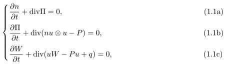
where n is the density，u=（u1，u2，u3）is the velocity，Π=（Π1，Π2，Π3）and Πj=nujis the momentum density，P=（Pij）3×3is the stress tensor，W is the energy density andis the heat flux and T is the temperature.This system also emerges from descriptions of the motion of the electrons in semiconductor devices，with the electrical potential and the relaxation omitted［4］.

In this paper，we consider the following case.The stress tensor is given by

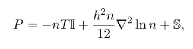
where I is the identity matrix and S is the viscous part of the stress tensor given by

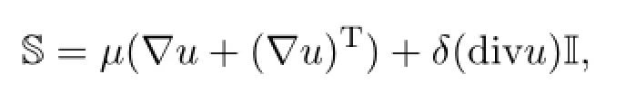
whereµ＞0 and δ are the primary coefficients of viscosity and the second coefficients of viscosity，respectively，satisfying 2µ+3δ≥0.The energy density W is given by

The quantum correction to the stress tensor was proposed by Ancona and Tiersten［2］on general thermodynamical grounds and derived by Ancona and Iafrate［1］in the Wigner formalism.The quantum correction to the energy density was first derived by Wigner［14］.See also［5］.With these quantum corrections（ħ＞0），system（2.7）is called the compressible quantum Navier-Stokes（CQNS）equations.When ħ=0，it reduces to the standard compressible Navier-Stokes（CNS）equations and was studied by Matsumura and Nishida［9］for the existence of smooth small solutions.

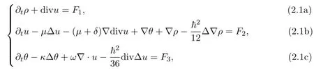
Obviously，（n，u，T）=（1，0，1）is a solution for（2.7）.To show the existence of small solutions near（1，0，1），we consider（ρ，u，θ）=（n-1，u，T-1）and transform（2.7）into the following quantum hydrodynamic equation

Recently，we obtained the following global existence result of small smooth solutions in［12］.

Theorem 1.1 Let s≥3 be an integer.Assume that（ρ0，u0，θ0）∈Xsfor s≥3. There exist positive constants ħ0，ε0，C0＞0 and ν0＞0 such that if ħ≤ħ0and

then the Cauchy problem（1.2）has a unique solution（ρ，u，θ）globally in time satisfying

for any t≥0.

In this paper，we consider the decay of the solutions constructed in Theorem 1.1 to the constant solution（ρ，u，θ）=（0，0，0）.The main result is stated in the following.

Theorem 1.2 Let ε0be the constant defined in Theorem 1.1 and s≥5.There exist constants ε1∈（0，ε0）and C＞0 such that for any ε≤ε1，if

and（ρ0，u0，θ0）∈L1（R3），then the solution（ρ，u，θ）in Theorem 1.1 enjoys the estimates

and

The decay rate is optimal in the sense that it is consistent with the linear decay rates in Theorem 2.1.To the best of our knowledge，there is no decay estimates for the compressible quantum Navier-Stokes equations（1.2），although there are some decay estimates to related models.For example，Matsumura and Nishida［8］studied the decay for the full Navier-Stokes equations and recently Wang and Tan［13］studied the optimal decay rates for the compressible fluid models of Korteweg type.See also［3，6，7，10，11］and the references therein.

In the next section，we consider the linear decay estimates for（1.2），and in the last section，we consider the nonlinear decay estimates and complete the proof of Theorem 1.2.

2　Linear Decay Estimates

In this section，we consider the Lq-Lpestimates of solutions for the Cauchy problem to the linearized system in R3.

2.1Reformulation

We rewrite（1.2）in the following

where

Take a linear transform of parameters

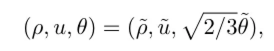
and set

with the initial data（ρ0，u0，θ0）.

Let A be the following matrix-valued differential operators

System（2.3）can be rewritten in an abstract form

where U=（ρ，u，θ）and F=（F1，F2，F3）.Then the corresponding semigroup generated by the linear operator-A is E（t）=e-tAfor t≥0.Then problem（2.4）can be rewritten in the integral form

2.2Linear decay estimates

To consider the decay of the linearized system，we consider the following abstract homogeneous equation

where U=（ρ，u，θ）and F=（f1，f2，f3）.Note that F here is different from that in（2.4）.

By taking Fourier transform of（2.6）w.r.t.space variable and then solving the ODE，we obtain

where F-1denotes the Fourier inverse transform andis the 5×5 matrix of the form

Theorem 2.1 Let E（t）be a solution operator of（2.6）defined by（2.7）.Then，we have the decomposition

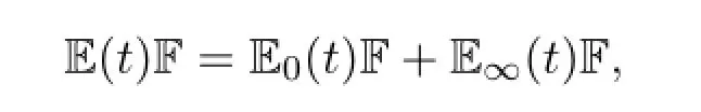
where E0（t）and E∞（t）have the following properties：

（1）For any integers m，l≥0，

where 1≤q≤2≤p≤∞；and

where 1≤q≤p≤∞and（p，q）/=（1，1），（∞，∞）.

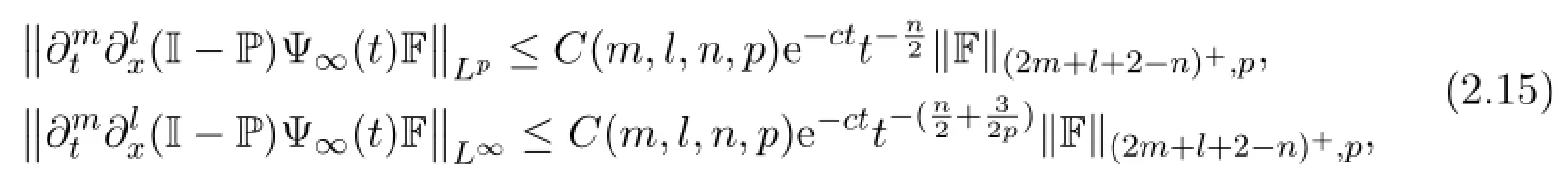
（2）Set（l）+=l if l≥0 and 0 if l＜0.For any 1＜p＜∞，there exists a c＞0 such that for any integers l，n≥0，

for all t＞0.

（3）Let 1＜p＜∞，then

for a suitable constant c＞0，for all t＞0.

To prove Theorem 2.1，we shall first consider the following stationary problem in R3with a complex parameter λ，

By taking Fourier transform，we obtain

where

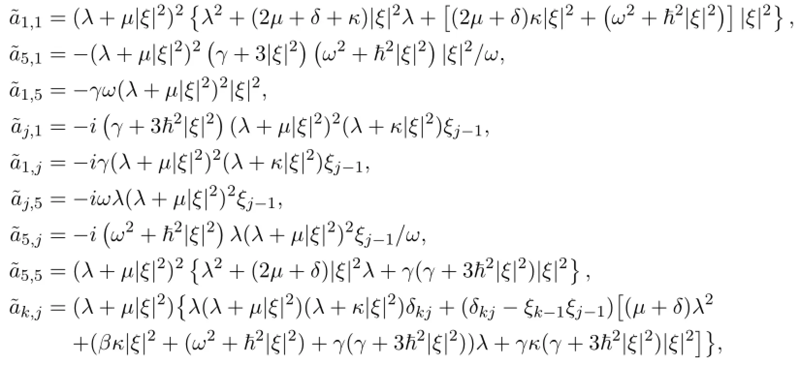
where k，j=2，3，4.

（1.a）There exists a positive constant r1＞0 such that λj（ξ）has a Taylor series expansion for|ξ|＜r1as follows

（1.b）Similarly，there exists a positive constant r2（＞r1）such that λj（ξ）has a Laurent series expansion for|ξ|＞r2as follows.Let ħ=o（1），then we have

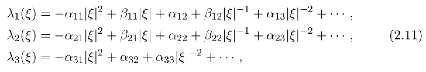
where α31＞0 is real depending only on the parameters and either（i）α11＞0 and α21＞0 are different real numbers or（ii）α11and α21are complex conjugates andℜα11=ℜα21＞0.In the first case，βij=0 for all i，j≥1.

（2）The matrix exponential has the spectral resolution

for all|ξ|＞0 except for at most four points of|ξ|＞0.

（3）For any 0＜R1＜R2＜∞，we have

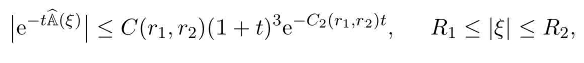
where C2＞0.

Sketched proof We need only to consider the proof of（1.b）.Let λ（ξ）be an eigenvalue written in Laurent series for large ξ.The coefficient A before|ξ|2then should satisfy the following algebraic equation

It is difficult to give exact expressions for A.But since ħ≪1，there is at least one negative solution A3=-α31＜0.For this，one can show that the eigenvalue hasthe form λ3（ξ）in（2.11）.For the other two roots of（2.12），either A1and A2are different real numbers，or A1and A2are complex conjugates（possibly with zero imaginary part）.When A1and A2are different real numbers，the eigenvalues λ1（ξ）and λ2（ξ）both have the form

When A1and A2are complex conjugates，the eigenvalues λ1（ξ）and λ2（ξ）both have the form

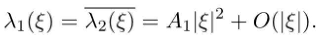
Since ħ≪1，the eigenvalues are small perturbations of the eigenvalues in the case when ħ=0 and hence ℜAj＜0 for j=1，2.We note that when ħ=0，the roots of（2.12）can be exactly solved to be A1=-（2µ+δ），A2=-κ and A3=0（see［6］）. The proof is completed.

Proof of Theorem 2.1 Let φ0（ξ）be a function insuch that φ0（ξ）=1 forandforand set

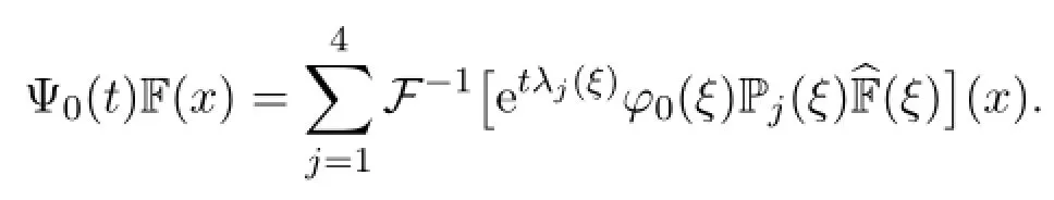
Since in the lower mode regime，the eigenvalues as well as the projectors behaves exactly as those in［6］，one obtains by the same treatment that

Next，we consider the high frequency part for large|ξ|.Let

where φ∞is a function insuch thatandforSet

We write

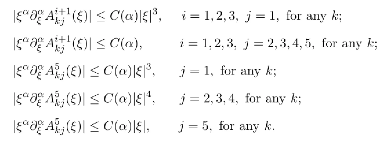
Let us consider first that α11and α21are positive real numbers in（2.11）.In this case，we obtain

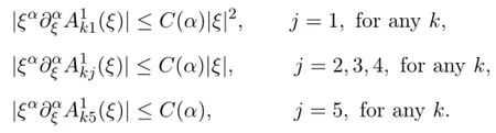
First，we have

for t＞0，1＜p＜∞，for any k∈｛1，2，3｝and j∈｛1，2，3，4，5｝.For the L∞-norm，we have

for t＞0，1＜p＜∞，for any k∈｛1，2，3｝and j∈｛1，2，3，4，5｝.Summarizing these estimates，we have proved the following

where（I-P）F=（f1，0，0，0，0）Tand PF=（0，f2，f3，f4，f5）T.

Now，we treat the estimates of PU.We write

It can be estimated that

Therefore we have proved the following

where（I-P）F=（f1，0，0，0，0）Tand PF=（0，f2，f3，f4，f5）T.

Choose φM（ξ）∈C∞0such that φ0（ξ）+φM（ξ）+φ∞（ξ）=1 for all ξ∈R3and set

Then it is easy to see that

for a suitable constant c＞0.Combining these estimates，we complete the proof of Theorem 2.1.

3　Nonlinear Decay Estimates

In this section，we shall prove two basic inequalities.

Lemma 3.1 Let U be a solution to problem（2.4）.Under the assumptions of Theorem 1.2，we have

Proof From Theorem 2.1 and（2.5），we have

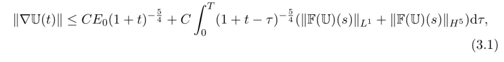
where F（U）is given in（2.2）.It follows from（2.2），H¨older inequality，Theorem 1.1 and Sobolev inequalities that

and similarly，

Combining these inequalities together completes the proof.

Lemma 3.2 Let U be a solution to problem（2.4）.Under the assumptions of Theorem 1.2，we have

Proof The proof is similar to Proposition 3.2 in［12］，and hence omitted here for simplicity.We only note that here，we require s≥6 while s=3 in Proposition 3.2 in［12］.The proof is completed.

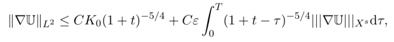
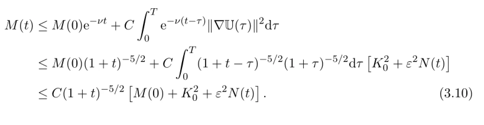
Proof of Theorem 1.2 Note that from（3.4），we have

for some constant D＞0.Definethen

From Lemma 3.1，we obtain

where we have used the following inequality［3］

where r1＞1 and r2∈［0，r1］and C（r1，r2）=2r2+1/（r1-1）.From Lemma 3.2 and Gronwall inequality，we have

By the definition of N（t），we obtain

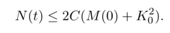
It then follows from the definition of N（t）that

In particular，

Next，we consider the Lp-decay of U.DenoteFirst of all，we have by letting m=0 in Theorem 2.1 that

From（2.4），we have

On the other hand，from（2.2），it is immediate that

It then follows from（3.12）that

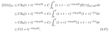
where 2≤p≤6 and 1≤q＜6/5 to insure application of（3.9）.This completes the proof.

Acknowledgment This work was initiated during the visiting of X.P.to Institute of Applied Physics and Computational Mathematics and the first author thanks for their hospitality.

References

［1］M.G.Ancona and G.J.Iafrate，Quantum correction to the equation of state of an electron gas in semiconductor，Phys.Rev.B，39（1989），9536-9540.

［2］M.G.Ancona and H.F.Tiersten，Macroscopic physics of the silicon inversion layer，Phys.Rev.B，35（1987），7959-7965.

［3］R.Duan，S.Ukai，T.Yang and H.Zhao，Optimal convergence rates for the compressible Navier-Stokes equations with potential forces，Math.Models Meth.Appl.Sci.，17：3（2007），737-758.

［4］C.L.Gardner，The quantum hydrodynamic model for semiconductor devices，SIAM J. Appl.Math.，54：2（1994），409-427.

［5］A.Jungel，J.-P.Milisic，Full compressible Navier-Stokes equations for quantum fluids：derivation and numerical solution，Kinetic and Related Models，4：3（2011），785-807.

［6］T.Kobayashi and Y.Shibata，Decay estimates of solutions for the equations of motion of compressible viscous and heat-conductive gases in an exterior domain in R3，Commun. Math.Phys.，200（1999），621-659.

［7］H.Li，A.Matsumura and G.Zhang，Optimal decay rate of the compressible Navier-Stokes-Poisson system in R3，Arch.Rational Mech.Anal.，196（2010），681-713.

［8］A.Matsumura and T.Nishida，The initial value problem for the equations of motion of compressible viscous and heat-conductive fluids，Proc.Japan Acad.Ser.A，55（1979），337-342.

［9］A.Matsumura and T.Nishida，The initial value problems for the equations of motion of viscous and heat-conductive gases，J.Math.Kyoto Univ.，20：1（1980），67-104.

［10］G.Ponce，Global existence of small solutions to a class of nonlinear evolution equations，Nonl.Anal.TMA.，9（1985），339-418.

［11］X.Pu and B.Guo，Global existence and convergence rates of smooth solutions for the full compressible MHD equations，Z.Angew.Math.Phys.，64（2013），519-538.

［12］X.Pu and B.Guo，Global existence and semiclassical limit for quantum hydrodynamic equations with viscosity and heat conduction，arXiv：1504.05304，Submitted.

［13］Y.Wang，Z.Tan，Optimal decay rates for the compressible fluid models of Korteweg type，J.Math.Anal.Appl.，379（2011），256-271.

［14］E.Wigner，On the quantum correction for thermodynamic equilibrium，Phys.Rev.，40（1932），749-759.

（edited by Liangwei Huang）

∗This work was supported in part by NSFC（11471057），Natural Science Foundation Project of CQ CSTC（cstc2014jcyjA50020）and the Fundamental Research Funds for the Central Universities（Project No.106112016CDJZR105501）.

†Manuscript received April 1，2016

‡Corresponding Author.E-mail：xuekepu@cqu.edu.cn