Determination of frequencies of oscillations of cloud cavitation on a 2-D hydrofoil from high-speed camera observations*

Patrik ZIMA， Tomáš FÜRST， Milan SEDLÁŘ， Martin KOMÁREK， Rostislav HUZLÍK

1. Institute of Thermomechanics of the CAS， v. v. i.， Prague， Czech Republic， E-mail:zimap@it.cas.cz

2. Faculty of Science， Palacký University in Olomouc， Olomouc， Czech Republic

3. Centre of Hydraulic Research， Lutín， Czech Republic

4. Faculty of Electrical Engineering and Communication， Brno University of Technology， Brno， Czech Republic



Determination of frequencies of oscillations of cloud cavitation on a 2-D hydrofoil from high-speed camera observations*

Patrik ZIMA1， Tomáš FÜRST2， Milan SEDLÁŘ3， Martin KOMÁREK3， Rostislav HUZLÍK4

1. Institute of Thermomechanics of the CAS， v. v. i.， Prague， Czech Republic， E-mail:zimap@it.cas.cz

2. Faculty of Science， Palacký University in Olomouc， Olomouc， Czech Republic

3. Centre of Hydraulic Research， Lutín， Czech Republic

4. Faculty of Electrical Engineering and Communication， Brno University of Technology， Brno， Czech Republic

A method is presented to determine significant frequencies of oscillations of cavitation structures from high-speed camera recordings of a flow around a 2-D hydrofoil. The top view of the suction side of an NACA 2412 hydrofoil is studied in a transparent test section of a cavitation tunnel for selected cloud cavitation regimes with strong oscillations induced by the leading-edge cavity shedding. The ability of the method to accurately determine the dominant oscillation frequencies is confirmed by pressure measurements. The method can resolve subtle flow characteristics that are not visible to the naked eye. The method can be used for noninvasive experimental studies of oscillations in cavitating flows with adequate visual access when pressure measurements are not available or when such measurements would disturb the flow.

unsteady cavitation， oscillation frequency， high-speed camera observation

Introduction

Unsteady cavitation phenomena are often studied using high-speed camera images of the liquid flow. Such visual observations provide useful qualitative information about the macroscopic cavitation structures［1，2］and are supported by quantitative measurements of the static pressures［3，4］， the local velocity field［5-8］and the high-frequency pressure oscillations［9，10］. Highspeed camera observations， however， can also be used to obtain valuable quantitative data on the cavitation phenomena and the underlying flow［9，11-13］. In Refs.［11］and ［13］ the brightness thresholding technique was employed to recognize cavitation regions in two- and three-bladed axial pumps from images obtained by a high-speed optical system for the characterization of flow instabilities generated by cavitation. The system is suited for the quantitative analysis of rotating cavitation instabilities in turbopump inducers and enabled the investigators to determine the tip cavity length and the frequency of the cavity length oscillation.

The ability to retrieve quantitative information from visual observations of cavitation is invaluable，especially when more traditional quantitative measurement methods are impossible to use due to geometric constraints， interference with the flow， excessive flow aggressiveness， or the rotation of the studied model. This paper presents a method of post-processing the experimental results of the comprehensive research carried out in the water cavitation tunnel in the Centre of Hydraulic Research， Lutín， the Czech Republic， on a prismatic NACA 2412 hydrofoil， in order to identify the cavitation-induced flow instabilities and their frequencies for a range of flow regimes and compare them with the CFD analysis. In order to minimize the interference with the flow and with respect to the small thickness of the foil， only two pressure transducer tap holes were accommodated at the hydrofoil midspan to measure the oscillations of the static pressure. The proposed method allows us to recognize the visible cavitation regions and perform their frequency analysis. It is used to determine the oscillations of the cavitation structures on the suction side of the hydrofoil and the results are compared withthe pressure oscillations measured by the tap hole on the suction side. It also helps to reveal flow characteristics which are not visible to the naked eye. The method is based on evaluating the brightness of the pixels in the digital images from the top-view highspeed camera， however， no threshold for the brightness is applied and the whole gray scale is considered in the analysis. We will demonstrate that such an approach can provide the benefit of a better resolution of the dominant oscillations and disclose more subtle oscillation frequencies.

Fig.1（a） Schematic of the cavitation tunnel in the closed water loop in the Centre of Hydraulic Research， Lutín，Czech Republic

Fig.1（b） Position of the high-speed digital video camera during experiment

1. Methods

1.1 Experimental setup

The pressure measurements and high-speed video recording were performed in the water cavitation tunnel in the Centre of Hydraulic Research in Lutín，Czech Republic. The set-up is described in Ref.［14］. Here， only the basic information on the set-up is provided. The tunnel is of the closed-loop type （Fig.1（a））and the test section with the rectangular cross-section has the inner dimensions of 0.15 m×0.15 m×0.5 m（width×height×length）. All the walls of the test section are made of organic glass to facilitate visualization from all sides （Fig.1（b））. The volume flow rate through the test section is measured by the magnetic inductive flow meter with an accuracy class of 0.3% located in the piping downstream of the main axial-flow pump of the tunnel. The maximum flow rate through the tunnel is 0.56 m3/s， which corresponds to the maximum velocity of 25 m/s at the inlet of the test section. The compressor and vacuum pumps installed above the water level in the reservoir are used to generate different pressure levels while maintaining a constant volumetric flow rate. The volume of the reservoir is 35 m3. The temperature of the water is measured in the reservoir by a platinum thermometer and the setup includes a bypass section for monitoring of the nuclei content by Acoustic Bubble Spectrometry.

The water from the reservoir enters the tunnel through the circular piping （DN 0.3 m） with a round mouth （inset of Fig.1（a））. The piping mouth is located inside the tank， sufficiently far from the wall， behind the tank soothing screens. The contraction ratio of the mouth based on the diameters of contraction （0.39 m: 0.3 m） is 1.69， however， the effective contraction ratio due to the flow contraction in the reservoir is expected to be higher. The piping is followed by the confusor reducing the DN 0.3 m cross-section to the square section 0.15 m×0.15 m and is 1.85 m long. The contraction ratio of the confusor is 3.14. Therefore， the total contraction ratio of the piping between the reservoir and the test section is 5.3 or higher. Different types of honeycombs can be inserted between the DN 300 pipe and the confusor to calm the flow. In this study， no honeycomb was installed.

The uniformity of the flow inside the test section（defined as the variation of the local velocity outside the boundary layer from the mean velocity） as determined from the CFD analysis is

The diffuser at the outlet of the test section expands the cross-section back to the circular DN 0.3 m and is 0.80 m long. The diffuser angle measured between from the pipe axis and the flat triangular walls（see Fig.2） isIn terms of equivalent crosssection radii the diffuser angle would be

The currently tested NACA 2412 hydrofoil is prismatic， with a chord length of 0.12 m， which gives a span-to-chord ratio of 1.25. The hydrofoil is made of stainless steel and is equipped with two circular tap holes connected non-invasively to pressure transducers located outside of the test section. The first tap hole，denoted by P0 （see Fig.2）， is located at the leading edge. The second tap hole， denoted by P40， is located on the suction side of the hydrofoil at 40% of the chord length. The diameter of the tap holes is 0.001 m and the openings are flush with the hydrofoil surface. The pressures were measured with a sampling freque-ncy of 5 kHz， with each record lasting 10 s. The accuracy of the transducers is 0.5 kPa. The small number of pressure transducers was chosen in order to minimize the influence of the holes on the flow in the regimes with high cavitation intensities. The PVDF hydrophone， denoted by P105， is located downstream of the hydrofoil trailing edge （at 105% of the chord length）. It measures high-frequency pressure pulses generated by the collapsing bubble clouds. The hydrophone is located outside of the region of interest of the present method and is only mentioned for completeness. In the following analysis， only pressure P40 will be considered.

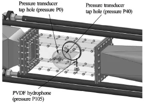
Fig.2 Schematic of the test section with circular windows enabling rotation of the hydrofoil and the NACA 2412 hydrofoil with two pressure transducers. The positions of the pressure transducer tap holes and the PVDF hydrophone are indicated by arrows

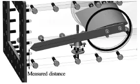
Fig.3 Principle of the incidence angle setting. The hand rotates along with the hydrofoil and the sharp tip of the hand indicates the distance from the bottom of the test section at a given horizontal distance from the rotation axis of the hydrofoil

The incidence angle of the hydrofoil was set tousing a removable hand with a sharp tip attached to the hydrofoil body and the rotating circular window of the test section using two screws （see Fig.3）. The tip of the hand is 0.234 m from the rotation axis of the hydrofoil. The distance between the hand tip and the bottom edge of the test section was measured using a micrometer ruler. The accuracy of the incidence angle setting was estimated to be about based on the accuracy of the distance measurement and the manufacturing tolerances of the components involved in the incidence angle setting. The accuracy of the setting repeatability was. The selected incidence angle enabled the flow to exhibit a range of cavitation regimes including the cloud cavitation regime with low-frequency periodic shedding of the sheet cavity and coherent collapses of bubble clouds.

The visualizations are obtained by a high-speed digital camera， recording the hydrofoil from the top. Each video record captures one second of the flow with a frame rate of 3 000 fps and a resolution of 1 024×672 pixels. The pressure measurements are synchronized with the camera.

Fig.4 Combination of the Reynolds and cavitation numbers used in the experiments with 4 different cavitation regimes.is the hydrofoil chord length，is the maximum leading-edge cavity length

The different cavitation regimes are achieved by setting the flow rate by the variable-speed driven axial-flow pump and the pressure in the water reservoir. The cavitation regime is determined by the Reynolds number and the cavitation number. The Reynolds number is defined as

Fig.5 Side and top views of the NACA 2412 hydrofoil with cloud cavitation. The flow is from left to right. The location of the P40 tap hole is denoted by a small arrow in the side view （The actual tap hole is located at midspan）

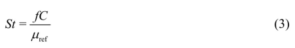
The oscillatory character of the flow is described by the Strouhal number defined as

1.2 Image processing tools

The video processing was performed in MATLAB with the Image Processing Toolbox［16］. Standard image processing techniques were used， including image filtering and image segmentation. The video recordings were processed into several time series of flow characteristics （see the results section）which were further analyzed by means of the Image Processing Toolbox， mainly to extract their dominant frequencies.

2. Results and discussion

Figure 4 shows the combinations of the Reynolds and cavitation numbers used in the experiments （total of 77 measurements representing 28 unique combinations of the nominal values ofReandσ）. For each of the 77 data points in Fig.4（a） high-speed camera recording （1 s long at 3 000 fps） was acquired and synchronized with the P0 and P40 pressure measurements. For the purpose of this study the groups of points obtained for the same nominal values are not averaged since only selected data points are used to demonstrate the function of the presented method. Besides this， the discussion of all 77 measurements is out of the scope of this study， which is focused on the presented method of data evaluation. For the purpose of this study， we have selected 2 representative regimes （see “analysis of high-speed camera images”below） with periodic cloud cavity shedding in order to demonstrate the strength of the method as compared to the pressure measurements.

The temperature of the water in the tunnel was betweenandfor all the experiments. The nuclei content in the tunnel was determined in a separate experiment using the dynaflow acoustic bubble spectrometer （ABS） installed in a removable bypass piping upstream of the convergent part of the test section. The range of the bubble radii measured by the ABS system was 15 µm-104 µm and the bubble volume fraction was 0.002% （which is rather high）.

The points in Fig.4 represent four different regimes including:

（1） he non-cavitating regime （the lowestand the highest cavitation number），

（2） the partial cavitation regime with a small oscillating leading-edge sheet cavity and no visible cavity shedding （high cavitation numbers），

（3） the cloud cavitation regime with the periodic shedding of the leading-edge sheet cavity （the maximum leading-edge cavity length ≤ hydrofoil chord length）， and

（4） the cloud cavitation regime with the end of the leading-edge sheet cavity intermittently extending downstream of the trailing edge （the maximum cavity length > hydrofoil chord length） （the highestand lowest cavitation numbers）.

Steady supercavitation has not been achieved in the experiments. The structure of the typical flow with the leading-edge sheet cavity shedding is illustrated in Fig.5 showing the side and top views of the test section recorded by high-speed digital cameras. The position of the P40 tap hole is denoted by the small arrow in the side view. As the sheet cavity grows， it covers the P40 tap hole resulting in a drop of the measured pressure. The pressure P40 is recovered temporarily when the sheet cavity is collapsed and the bubble cloud is shed towards the hydrofoil trailing edge. The whole cycle is repeated periodically with a frequency depending on the flow parameters. For the purpose of our analysis， we will select regimes with stable oscillations of the leading-edge sheet cavity over the P40 tap hole. Here， a stable oscillation is defined by the periodic appearance and disappearance of the leading edge cavity over the P40 tap hole. This selection will enable us to validate the presented method using the P40 pressure measurement.

Fig.6 Pressure readings at P40 tap hole for cloud cavitation regime with strong sheet cavity oscillationsThe frequency of the dominant oscillations is 15.3 Hz

The results of the P40 pressure measurements（tap hole on the suction side at 40% of the hydrofoil chord length） are shown in Figs.6-8. Figure 6 shows the pressure reading forandThe sheet cavity in this regime is highly unstable and oscillates with strong periodicity. A closer look at Fig.6 reveals that the time period of oscillation is，however， not perfectly constant and fluctuates approximately withinof the average value. The corresponding power spectrum of the pressure reading is shown in Fig.7. The dominant frequency of 15.3 Hzcan easily be observed， together with its higher harmonic partials.

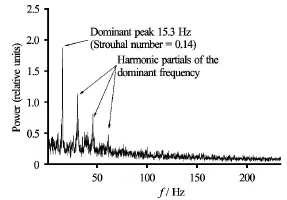
Fig.7 Fast Fourier Transform of 5 series of 10 s P40 pressure transducer readings （50 s of measurement） for the regime of strong sheet cavity oscillation1.8）. The dominant frequency of 15.3 Hzis easily observed， together with its higher harmonic partials

Fig.8 Intensity of the pressure oscillation expressed using RMS of the P40 pressure oscillations as a function of the cavitation number for different Reynolds numbers. The symbols denote discrete measurements， whereas the lines connect the average values of the measurements obtained for the same combination of nominaland

Figure 8 shows the standard deviation of the pressure oscillations across the whole frequency spectrum of the measured static pressure P40. It can be seen that for higher cavitation numbers （lower cavitation intensities） the pressure oscillations are only moderate. In these regimes the leading-edge sheet cavity does not reach the P40 tap hole. As the cavitation number is decreased for a fixed Reynolds number， the end of the leading-edge sheet cavity reaches the position of the P40 tap hole and the severity of the oscillations increases significantly. As the cavitation number is decreased further， the sheet cavity is extended towardsthe hydrofoil trailing edge and the pressure oscillations drop back to modest values. The regime shown in Figs.6 and 7 is represented by the peak value of the data in Fig.8 for the highest Reynolds number examined （1.7×106）.

3. Analysis of high-speed camera images

In the following section， we will explain our method by analyzing the cavitation regime withand（shown in Figs.6 and 7）. We will also use the method to analyze the regimeandto demonstrate its ability to determine a secondary frequency besides the dominant frequency of oscillation. The two regimes were selected to ensure that the leading-edge cavity oscillated over the P40 pressure transducer tap hole. This way the results obtained by the presented method can be tested against the pressure measurements. Once the agreement with the pressure measurements is confirmed， the method can be used to analyze the frequency characteristics of a wide range of cavitation regimes including the ones where the leading-edge cavity does not extend to the P40 tap hole.

The first regime of our interest， i.e.，and， is characterized by stable oscillations of the leading-edge sheet cavity and the cavity oscillates over the position of the P40 tap hole. This will enable us to compare the image analysis with the P40 pressure measurements. The development of the sheet cavity lasts approximately 0.05 s and is followed by its rapid collapse， which takes less than 0.01 s. The collapse produces secondary bubble clouds， which travel downstream and the whole process repeats.

Fig.9 The region of interest above the central part of the foil

We proceed as follows. First， to exclude the effect of the three-dimensional flow at the sidewalls of the test section， we concentrate on a rectangular area above the hydrofoil， positioned at midspan around the axis of symmetry （dashed line in Fig.9）. The deformation of the images from the high-speed camera due to the small departure of the camera lens axis from the vertical axis is neglected. This is justified because the contribution of the deformation to the studied quantities is insignificant. The region of interest （ROI） is 60 pixels wide （in the span-wise direction） and 438 pixels long （in the chord-wise direction）， which corresponds to approx. 0.016 m×0.119 m （the hydrofoil chord length is 0.12 m， however， due to the incidence anglethe chord appears 0.001 m shorter in the plan view）. Some care must be taken with the selection of the ROI width. This will be discussed later in this section. For the time being， the ROI width is set to a value of 60 pixels. At each time point， the ROI is cropped， the background （i.e. an image with no cavitation structures） is subtracted from it， and the columnwise average （i.e.， in the span-wise direction） of the pixel values on the 0-255 grayscale is computed. The grayscale value of 0 represents no cavitation and 255 represents the maximum brightness of the cavitation region. Thus， at each time， a vector of 438 average values is produced. When the entire video （lasting 1 s and containing 3 000 frames） is processed， a 3 000× 438 matrix of average brightness values is produced.

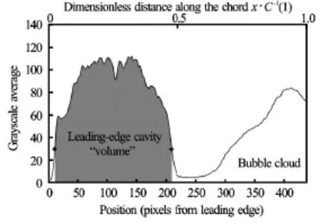
Fig.10 Average grayscale values along the chord of the region of interest at a fixed time （chord length）. The two main ridges in the image are separated by a “valley” of darker pixels. The two stars delimit the boundaries of the first ridge as determined by the automatic procedure.is the coordinate along the chord（from the leading edge）

In order to separate the oscillation frequencies of the leading-edge sheet cavity from the effect of the fast moving bubble clouds （see the right part of Fig.5），we will explore two approaches for the method:

（1） At each time instant， we attempt to identify two “ridges” in the averaged signal. This situation is illustrated in Fig.10. The first ridge， closer to the leading edge， is attributed to the presence of the leading-edge sheet cavity. The second ridge， closer to the trailing edge， is attributed to the bubble clouds. The two ridges are separated by a “valley” of darker pixels. When the first ridge is identified （at certain time instants， only this first ridge may be present） its area under the curve of the grayscale averages is computed. This area is then taken to be a proxy for the sheet cavity volume. The identification of the first ridge is fullyautomatic and is implemented as a simple threshold procedure. The threshold was set to a value of 30. This was roughly twice the average of the values in the “valley” between the first and second ridge. The time series of the first ridge volumes is then run through a median filter to remove occasional inaccuracies in the identification of the right boundary of the first ridge.

（2） For each position along the chord we take the average of the grayscale values of the 60 pixel vertical dimension of the region of interest. This produces a time series for each position. This series is analyzed and its first autocorrelation maximum is found. The position of this maximum defines the dominant frequency at the given position along the chord and its amplitude defines the relative magnitude of the oscillations.

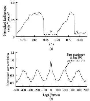
Fig.11 （a） An excerpt from the time series of the leading-edge cavity “volume” （measured by the area under curve between the two stars in Fig.10）. The “volume” is normalized between 0 and 1 so that the largest identified cavity has the volume of 1. Notice the sharp drops that correspond to the collapse of the sheet cavity. This is the dominant mechanism responsible for the observed pressure oscillations. （b） A detail of the autocorrelation structure of the time series of the sheet cavity “volume”. The dominant frequency is found to be 15.3 Hz（St=. One time frame corresponds to 1/3 000 s

For both approaches outlined above the time series of the investigated quantity （cavity “volume”for approach （1） and the grayscale average for approach （2） is analyzed to find its autocorrelation structure. The autocorrelation functionis computed from the following formula where the investigated quantityis zero-padded.is the signal length，is the summing index，is the signal shift.

We will now proceed with approach （1） explained above. First， we will explain the term “lag” used as the unit on the horizontal axes in Figs.11（b）， 12（a），14 and 15. Each video consisted of 3 000 frames capturing 1 s of the flow. Thus， the lag between the successive frames is 1/3 000 s. Consequently， the lag offrames corresponds to the time difference of， which corresponds to the frequency

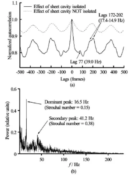
Fig.12 Flow regime withand. （a）Autocorrelation structure from the high-speed camera images. When the leading-edge cavity effect is isolated from the effect of bubble clouds （solid curve） a secondary oscillation frequency of 39.0 Hzis revealed. This frequency is not resolved when the leading-edge cavity effect is NOT isolated （dashed curve）.（b） FFT analysis of the signal averaged from two 10 s P40 pressure readings （total of 20 s）. A secondary frequency of 41.2 Hzcan be identified besides the dominant frequency 16.5 Hz

Figure 11（a） shows a typical temporal evolution of the first ridge volume. The time of the leading-edge sheet cavity development and the time of its collapse can be easily read from the curve. Figure 11（b） shows the autocorrelation structure of the first ridge volume. The dominant frequency is 15.3 HzThe experimentally measured pressure pulsation （see Fig.7）has the dominant frequency 15.3 Hz （15.26 Hz）. Thedifference of the frequencies lies comfortably within the experimental error.

It is worth noting that if we did not attempt to separate the primary bubble cloud and analyzed the time series of the area under the entire curve from Fig.10， the peak at 15.3 Hzwould still be clearly visible in Fig.11， however， it would be much less pronounced. The advantage of isolating the first ridge and excluding the second ridge （i.e.， isolating the leading-edge cavity effect from that of the bubble clouds） is documented in Fig.12（a） for the regime withand. The analysis with the identification of the first ridge reveals another frequency of 39 Hz， which is not captured when the second ridge is not excluded from the analysis. This frequency is clearly visible in the FFT analysis of the P40 pressure measurement for the regime shown in Fig.12（b）. The origin of the secondary frequency is unknown to the authors， however， it is captured by the pressure measurement and resolved by the presented method.

As we mentioned earlier， the gray area in Fig.10 is taken as the proxy of the sheet cavity volume. In reality， the image produced by the high-speed camera is a plan view of the cavity where the grayscale values of each pixel point in the view contribute to the total area. The notion of “volume” is therefore based on the assumption that the grayscale value of each pixel point is somewhat proportional to the physical volume of the cavity beneath the particular pixel point. As a result， the cavity is viewed as a body of non-uniform density （or thickness） with a continuous boundary rather than a body of constant density （or thickness）with a discrete boundary. Although this assumption is a simplification， it is a practical one because it allows us to estimate the cavity volume more accurately.

The relation between the “volume” changes of the sheet cavity and the measured pressure oscillations also requires some discussion. The pressure measurement only captures the local pressure oscillations at a single point in space. These oscillations might be a result of the superposition of different pressure effects present on the hydrofoil or in its vicinity. On the other hand， the cavity “volume” changes determined by the presented method are a representation of the global geometric oscillations of the whole sheet cavity. If the pressure tap hole， however， is located conveniently（i.e.， the sheet cavity fluctuates over the tap hole）， the measured pressures oscillations will exhibit the same frequencies as the cavity “volume” oscillations obtained by the presented method. The two cavitation regimes used in this study have been selected in order to ensure that the pressure measurements at position P40 can be used to validate the presented method.

Before we proceed to employing approach （2）described above we will discuss the dependence of the results from the post-processing of the high-speed camera images on the selection of the ROI width （as defined in Fig.9）. This dependence is shown in Fig.13 and is constructed as follows. For each ROI half-width（1-214 pixels） the mean grayscale value of all the pixels in the ROI is calculated and the value is averaged for all 3 000 frames of the selected high-speed camera video. The calculated mean brightness of the ROI is then normalized by the mean brightness of the 1-pixel ROI half-width to obtain the dimensionless mean brightness. The dependence of this quantity on the ROI half-width is then plotted for a number of different cavitation regimes. For a very small ROI half-widththe mean brightness is strongly dependent on the ROI size. For an exceedingly large ROI half-widththe mean brightness is most likely influenced by the effect of threedimensionality of the flow near the test section walls. The optimum range lies between 30 pixels and 90 pixels and should be determined separately for each different application. In our analysis， the ROI halfwidth of 30 pixels （i.e.， ROI width of 60 pixels） was used as an acceptable value for most cavitation regimes. Higher ROI widths can also be used （depending on the regime）， however， when the ROI width is increased the autocorrelation function such as the one shown in Fig.12（a） becomes “smoother” and smaller peaks are not resolved. For ROI widths close to the hydrofoil span the autocorrelation function becomes similar to the one obtained when the effect of the leading-edge cavity is not isolated from the other cavitation structures except that the amplitudes of the autocorrelation peaks are higher.

Fig.13 Sensitivity of the video analysis to the selection of the ROI width

We will now modify the presented method to explore approach （2） described above. The ROI width（in the span-wise direction） will remain 60 pixels，though the ROI length （in the chord-wise direction）will be reduced to 1 pixel. For each such ROI of 1×60 pixels the average grayscale value is calculated at each pixel position along the chord and the autocorrelation structure is determined for all 3 000 frames of the high-speed video. The results for the regime withand（shown also in Figs.6， 7 and 11） are plotted in Fig.14 for selected points along the chord （5%， 25%， 40%， 65%， 80%， and 95%）. Using this approach the dominant frequency of 15.3 Hz （3 000 frames/196 lags） can also be determined with great accuracy， though only for chord distances greater than 65%. This fact can be a consequence of the irregularities in the development and collapse of the leading-edge cavity （see Fig.11（a）） and the relative regularity of the shedding of the collapsed cavity towards the trailing edge.

Fig.14 Autocorrelation structure from the high-speed camera images for 6 different positions along the chord. The dominant frequency of 15.3 Hzcan be determined from the first autocorrelation maximum downstream of the 65% chord distance. Flow regime withand

Fig.15 Autocorrelation structure from the camera images at chord distance 100%. Secondary frequency 38.1 Hzcan be determined besides the dominant frequency of 16.1 Hz. Flow regime withand

Finally， we will test if approach （2） can reveal the secondary frequency about 39 Hz-40 Hz shown in Fig.12 for the regime withandFor this purpose only the pixel column at the trailing edge of the hydrofoil is considered （100% distance along the chord） and the result is shown in Fig.15. The secondary frequency of 38.1 Hzcan be determined in addition to the dominant frequency of 16.1 Hz. It is worth noting that secondary frequencies in the range 25 Hz-190 Hz appear in many other cavitation regimes shown in Fig.4 and that they are not higher harmonics of the primary （dominant）frequency. They can be revealed by both the pressure measurements as well as the presented method. We do not offer an explanation of the physical meaning of the frequencies here， however， they are a subject of an ongoing research into cavitation instabilities.

4. Conclusions

A computationally inexpensive method is presented to determine the dominant frequencies of oscillations of cloud cavitation on a 2-D hydrofoil from topview high-speed camera observations in a cavitation tunnel. In order to circumvent the effect of the flow three-dimensionality at the test section sidewalls and to ensure a sufficient resolution of the method， some care must be taken to select the region of interest. The grayscale image of the region of interest is analyzed at each time instant producing a time series of grayscale values along the chord at the hydrofoil midspan. Two modes of the method are considered: the first mode， in which the leading-edge cavity is identified and its size（or “volume”） is quantified in order to determine its size oscillations in time， and the second mode， in which the oscillations of the grayscale values at different fixed positions along the chord are analyzed. For both modes， the autocorrelation structure of the investigated quantity （either the leading-edge cavity “volume” or the pointwise grayscale values） is determined numerically using a fully automatic procedure. The position of the first autocorrelation maximum （the dominant frequency） corresponds to the frequency of cavity shedding or local cavity oscillations.

The frequencies determined by the presented method have been compared with the measurements of the static pressure on the hydrofoil for two selected regimes characterized by stable cloud cavity shedding yielding very good agreement. The two regimes were selected so that the leading-edge cavity oscillated across the pressure tap hole to ensure the pressure transducer captured the cavity oscillations. It has been shown that the method can also resolve flow characteristics in the form of subdominant frequencies that are not visible to the naked eye but captured by the pressure measurements. The physical origin of these secondary frequencies is under investigation. The method can be used for non-invasive experimental studies of oscillations in cavitating flows with adequatevisual access when pressure measurements are not available or when such measurements would disturb the flow.

The cavity “volume” changes determined by the presented method are a representation of the global geometric oscillations of the sheet cavity. A conveniently selected region of interest will capture the oscillation frequencies for the entire range of oscillatory cavitation regimes. In contrast， the pressure measurement point （or points） must be located conveniently for each cavitation regime in order to capture the dominant oscillation frequency （i.e.， not downstream of the oscillating cavity）. Besides this， the pressure measurement is invasive （it often influences the flow，especially near the leading edge）， the installation of pressure tap holes is expensive and limited by the space constraints， especially for thin foils. Any change of configuration of the pressure measurement requires the manufacturing of a new test foil. On the contrary，any changes of configuration of the presented method occur at the post-processing stage and can easily be achieved on the software level. On the other hand，the presented method requires visual access， a highspeed camera and a strong source of uniform illuminetion of the region of interest.

In this paper the presented method is applied to the problem of cavitation above a 2-D hydrofoil. After some modifications the method can be used for other problems and geometries with visual access to the cavitation region such as in oscillating cavitation nozzles and cavitation jets. Such configurations， however， have not been examined by the authors. For such purposes both modes of the presented method could be employed to study the global as well as the local oscillatory character of the cavitation regions. The modification would consist of a careful selection of the rectangular region of interest in the flow direction and in ensuring its uniform illumination and adequate camera frame rate. For rotating cavitation problems （assuming the use of a strobe light） the second mode of the presented method is not suitable and the first mode would require an updated algorithm of identification and quantification of the oscillating cavitation region. The analysis of the autocorrelation function， however， can be applied without significant changes.

Acknowledgements

This work was supported by the Czech Science Foundation （Grant No. 13-23550S）， the institutional support RVO:61388998 of the Institute of Thermomechanics of the CAS， v. v. i..

References

［1］ FRANC J. P.， MICHEL J. M. Fundamentals of cavitation［M］. Boston， China: Kluwer Academic Publishers，2004.

［2］ ARNDT Roger E. A. Some remarks on hydrofoil cavitation［J］. Journal of Hydrodynamics， 2012， 24（3）: 305-314.

［3］ DUTTWEILER M. E.， BRENNEN C. E. Surge instability on a cavitating propeller［J］. Journal of Fluid Mechanics，2002， 458: 133-152.

［4］ WATANABE S.， KONISHI Y. and NAKAMURA I. et al. Experimental analysis of cavitating behavior around a Clark Y hydrofoil［C］. WIMRC 3rd International Cavitation Forum. Coventry， UK: University of Warwick，2011.

［5］ FOETH E. J.， Van DOORNE C. W. and Van TERWISGA T. Time resolved PIV and flow visualization of 3D sheet cavitation［J］. Experiments in Fluids， 2006， 40（4）: 503-513.

［6］ KRAVTSOVA A. Y.， MARKOVICH D. M. and PERVUNIN K. S. et al. High-speed visualization and PIV measurements of cavitating flows around a semi-circular leading-edge flat plate and NACA0015 hydrofoil［J］. International Journal of Multiphase Flow， 2014， 60（2）: 119-134.

［7］ DULAR M.， BACHERT R. and SIROK B. et al. Transient simulation， visualization and PIV-LIF measurements of the cavitation on different hydrofoil configurations［J］. Journal of Mechanical Engineering， 2005， 51（1）: 13-27.

［8］ MORI T.， KIMOTO R. and NAGANUMA K. PIV measurements of propeller flow field in a large cavitation tunnel［C］. ASME-JSME-KSME 2011 Joint Fluids Engineering Conference. Fora， Hamamatsu， Japan， 2011，47-52.

［9］ CERVONE A.， TORRE L. and BRAMANTI C. et al. Experimental characterization of the cavitation instabilities in a two-bladed axial inducer［J］. Journal of Propul- sion and Power， 2006， 22（6）: 1389-1395.

［10］KAWANAMI Y.， KATO H. and YAMAGUCHI M. et al. Mechanism and control of cloud cavitation［J］. Journal of Fluids Engineering， 1997， 119（4）: 788-794.

［11］ CERVONE A.， BRAMANTI C. and TORRE L. et al. Setup of a high-speed optical system for the characterization of flow instabilities generated by cavitation［J］. Journal of Fluids Engineering， 2007， 129（7）: 877-885.

［12］ FOETH E. J.， Van TERWISGA T. and Van DOORNE C. On the collapse structure of an attached cavity on a threedimensional hydrofoil［J［. Journal of Fluids Engineering，2008， 130（7）: 071303.

［13］ CERVONE A.， BRAMANTI C. and TORRE L. et al. Characterization of cavitation instabilities in axial inducers by means of high-speed movies［C］. 42nd AIAA/ ASME/SAE/ASEE Joint Propulsion Conference and Exhibit， Joint Propulsion Conferences. Sacramento， California， USA， 2006.

［14］KOMÁREK M.， SEDLÁŘ M. and VYROUBAL M. et al. Preparation of experimental and numerical research on unsteady cavitating flow around hydrofoil［J］. EPJ Web of Conferences， 2015， 92: 02036.

［15］ COOPER J. Revised release on the IAPWS industrial formulation 1997 for the thermodynamic properties of water and steam［C］. The International Association for the Properties of Water and Steam. Lucerne，Switzerland， 2007， 1-48.

［16］ MATLAB. Image Processing Toolbox， Rel. 2013b［M］. MathWorks， Inc.， 2013.

October 3， 2015， Revised March 17， 2016）

* Biography: Patrik ZIMA （1972-）， Male， Ph. D.，

Research Scientist