
Time Finite Element Method for Initial Problem with Fractional Order Derivative
2017-04-19 05:49ZHENGYunyingZHAOZhengang
淮北师范大学学报(自然科学版) 2017年1期
ZHENG Yunying,ZHAO Zhengang
(1.School of Mathematical Sciences,Huaibei Normal University,235000,Huaibei,Anhui,China;2.Department of Fundamental Courses,Shanghai Customs College,201204,Shanghai,China)
Time Finite Element Method for Initial Problem with Fractional Order Derivative
ZHENG Yunying1,ZHAO Zhengang2
(1.School of Mathematical Sciences,Huaibei Normal University,235000,Huaibei,Anhui,China;2.Department of Fundamental Courses,Shanghai Customs College,201204,Shanghai,China)
In this paper,the time Galerkin finite element algorithm is formulated for a type of nonlinear time fractional differential equation.The existence and uniqueness are proven and priori error estimate for this algorithm are studied in detail.Numerical example for the nonlinear ordinary fractional equation with initial value are given which confirm the theoretical convergence rate.
Caputo derivative;fractional initial problem;time finite element method
0 Introduction
In this paper,we mainly discuss the model with initial value described as follows.

1 Fractional Derivative
In this section,we firstly introduce the fractional integral,fractional Caputo derivative and their properties.
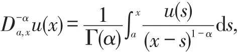
Definition 1 Theα-th order left and right Riemann-Liouville integrals of functionu(x)are defined as follows:
WhereCDβa,tdenotes fractional left derivative in the sense of Caputo.It is hard to get the analytical solution in spite of the simply form.So many researchers try their best to seek the numerical solution.
The Galerkin finite element method has many advantage in numerically solving differential equations,such as stability,flexibility of mesh and efficiency in shape functions.It has become a very attractive tool for classical parabolic problems and the second-order hyperbolic equations[1-3],etc.,and also was introduced to numerical treating the fractional differential equations,such as the partial derivative[4-8],etc.in the last decades.
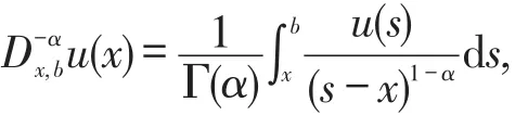
whereα>0anda<x<b.
Definition 2 Theα-th order Caputo derivatives of functionu(x)are defined as follows:
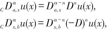
wheren-1<α<n∈Z+anda<x<b.
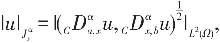
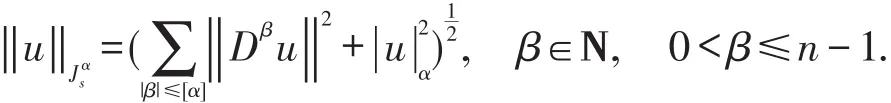
Definition 3 Letα>0,define a fractional spaceJsα,p(Ω),Jsα(Ω)={u∈Hn(Ω):CDαa,xu∈L2(Ω),CDαx,bu∈L2(Ω),n-1≤α<n}, endowed with the semi-norm
and the norm
LetJsα,0,C20αbe the closure of the spacesJsα,C2α,and give some useful results.
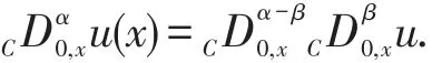
Lemma 1[6]Foru∈Jαs,0([a,b]),0<β<α,then
Lemma 2[8]Foru∈Jαs,0(Ω),0<β<α,then
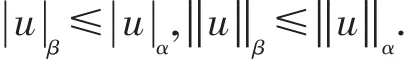
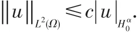
Foru∈Hα0(Ω),then
Lemma 3[7]Foru∈Jαs,0([a,b]),D-μ0,t:L2(Ω)→L2(Ω)is s bounded linear operator.
2 The Time Galerkin Finite Element Approximation
In this section we will formulate a time Galerkin finite element method for a type of nonlinear time fractional equation.
Problem 1 For0<β<1,

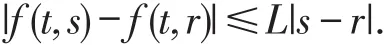
For the function fdefined on(0,T]×R,we have the following assumption:there exists a positive mild Lipschitz constantLsuch that fort∈(0,T],
Let us consider a partition ofI=(0,T].Set0=t0<t1<t2<…<tN=T be the subdivision ofI,and Ij=(tj,tj+1],kj=tj+1-tj,j=0,1,…,N-1.On each time slabIj,we define a discrete function spaceℑk
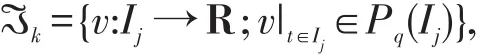
The functions ofℑkcan be discontinuous at the time nodetj,but it is left-continuous and right-continuous,and the functions ofℑkare polynomials,which numbers are no more thanq-1.
In order to derive a variational form of problem 1,we assume thatuis a sufficiently smooth solution of problem 1 and multiply by an arbitraryv∈ℑkto obtain the integration formulation:
for each time interval and any continuous test functionv,the solution to problem 1 with the initial valuesatisfies

So we simply write the time Galerkin finite element scheme as:findU∈ℑk,such that for allvinℑk,there has

In this paper,for each time slab,we plan to adopt the trial space as piecewise constant trial space.Thus for everyU∈ℑk,the following formula is achieved.

and also the following expression is hold.
this means we would not solve the solution at time nodeTn+1in time slabIn.In order to conquer this difficulty,we apply the property of the fractional derivative to dealt with the first term in the left hand of(3),and with the help of equality(4),we have
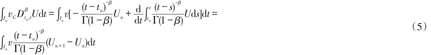
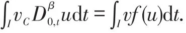
As to the second term,there are two methods to approximate.The first is to adopt the difference scheme in each time slabIi,i=0,1,…,n-1;the second is integrating by parts,change the derivative of functionu into a integration.
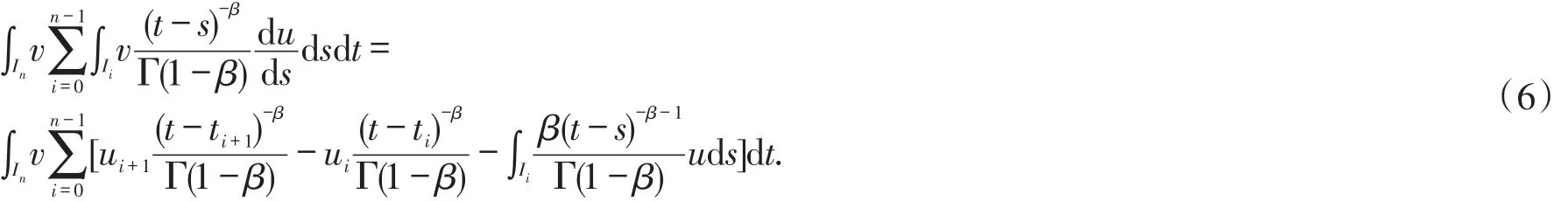
with above two relations(5)and(6),we give the specific scheme for the fractional initial problem(1)as the following form:findU∈ℑk,such that

for allvin ℑk.
Next we prove uniqueness for our numerical scheme.
Theorem 1 Assume that(M,k)is an p-discretization of(0,T],withckβ≤1,then there exists a unique time Galerkin finite element solutionU∈ℑk.
Proof of Theorem 1 Given the initial valuesU0,it is sufficient to show that the problem on time slab Inhas a unique solutionU|In∈Pq(In,R).To do so,we setU=Tis the solution of the following equation.

for allv∈Pq(In;R).Since the above system is a linear system,according to Banach fixed point theorem,there exists at least one solution,we set it asU=T.If the operatorT is compact,then with the fixed point theorem,there exists only one solution.To do so,we suppose there exists another solutionW=T,set E=U-Wand=-.TakeEandinto equation(8),with the same initial valueU0=W0,one has

next we estimate each term in the above equation.Setv=En+1,then


With estimations(10)and(11),we get

Summingnfrom 1 toN,and with the lemma 3,one has

So the following estimation can be gotten immediately.
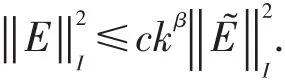
Whenckβ≤1,one has

It means that the operatorTis compact,so the existence and uniqueness are proven.
3 Error Estimation
Next we estimate the error bound.We denoteeis the error between approximation solutionUand exact solutionu,the formula among three solutions is given below:

wherePhUis the interpolation ofuin time domain,and satisfies thatPhU(ti)=ui,i=1,2,…,N.That means ρi=0at each time nodeti.
Theorem 2 Assume that(1)has a solutionusatisfying,u′∈L2(0,T).If(M,k)is an p-discretization of(0,T],then the time finite element approximation(7)is convergent to the solution(1)on the interval(0,T],ask→0.The approximation solutionUsatisfying the following error estimate

Proof of theorem 2 Minus(2)from equation(7)and introduce relation(15)into it,we have the following error equation.

Setv=θn+1,then the following estimations are derived.

Next we consider the first term in the right hand of equation(13).

the second term can be estimated as follow:
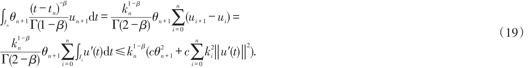
and withu0=U0,

The third term and fourth term satisfy the following estimations:

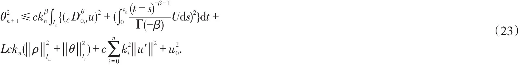
The last term in the right hand side of(16)is estimated below:

Together with(17)to(23),and sufficient smallkn,the result can be gotten.
Multiplyingknon the both side of above inequality,also with the sufficient smallknwe have

Summingnfrom 1 toN,with the relationU=θ+ρ+uand using the boundedness of fractional integral in lemma 3,we get

Whenkis sufficient small,the second term in the right hand of above estimation can be hidden in the left,so we have

With the properties of interpolation functionPh[6],the proof of theorem 2 is ended.
4 Numerical Examples
In this section,we present numerical results for the time finite element approximations which supports the theoretical analysis in section 3.
Example 1 We consideru(t)=t2-tas the exact solution of the following equation
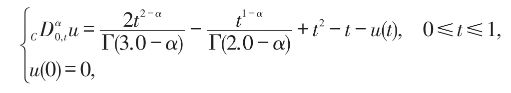
LetShdenote a uniform partition on[0,1],andXhthe space of piecewise constant functions onSh.We selectthen the following table is given.We can observe that the experimental rates of convergence near to 1,and it is better than the theoretical rate.The reason is in our numerical example,the initial value is homogeneous,the effect of initial value is omitted for the numerical solution.
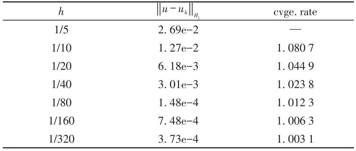
Table1 Numerical error results for Example 1 with α=β=0.5
[1]LASIS A,SÜLI E.Hp-version discontinuous Galerkin finite element method for semilinear parabolic problems[J].Siam J Numer Anal,2005,45(4):1544-1569.
[2]XU Y,SHU C W.Error estimates of the semi-discrete local discontinuous Galerkin method for nonlinear convection-diffusion and KdV equations[J].Comput Methods Appl Mech Engrg,2007,196:3805-3822.
[3]WANG K X,WANG H,SUN S Y,et al.An optimal-order L2error estimate for nonsymmetric discontinuous galerkin methods for a parabolic equation in multiple space dimensions[J].Comput Methods Appl Mech Engrg,2009,198:2190-2197.
[4]BRUNNER H,SCHÖTZAU D.Hp-discontinuous Galerkin time-stepping for Volterra integradifferential equations[J].Siam J Numer Anal,2006,44(1):224-245.
[5]MCLEAN W,MUSTAPHA K.Convergence analysis of a discontinuous Galerkin method for a sub-diffusion equation[J]. Numer Algor,2009,52(1):69-88.
[6]FIX G J,ROOP J P.Least squares finite-element solution of a fractional order wo-point boundary value problem[J]. Comp Math Appl,2004,48:1017-1033.
[7]ERVIN V J,ROOP J P.Variational formulation for the stationary fractional advection dispersion equation[J].Numer Meth Partial Diff Equ,2006,22:558-576.
[8]ZHAO Z G,ZHENG Y Y,GUO P.A Galerkin finite element scheme for time-space fractional diffusion equation[J].Int J Comp Math,2016,93(7):1212-1225.
一类分数阶初值问题的时间有限元算法
郑云英1,赵振刚2
(1.淮北师范大学 数学科学学院,安徽 淮北 235000;2.上海海关学院 基础部,上海 201204)
针对一类含有Caputo导数的分数阶非线性初值问题建立了一个时间有限元格式.运用压缩映像原理分析了格式的存在唯一性,并对时间有限元算法的误差估计进行详细讨论,数值例子表明,格式是可行的,数值收敛阶符合理论分析.
Caputo导数;分数阶初值问题;时间有限元
O 175.13
A
2095-0691(2017)01-0001-06
2016-11-18
安徽省自然科学基金项目(1408085MA14);国家自然科学基金项目(11301333);上海市教育委员会科研创新项目(14YZ165)
郑云英(1973- ),女,河北邢台人,博士,副教授,研究方向:分数阶微分方程数值解.
O 175.13 Document Code:A Article ID:2095-0691(2017)01-0001-06
Received date:2016-11-18
This work was supported by Natural Science Foundation of Anhui Provence Under Grant(1408085MA14);The National Natural Science Foundation of China Under Grant(11301333);The Innovation Program of Shanghai Municipal Education Commission Under Grant(14YZ165)
Author:ZHENG Yunying(1973- ),female,hail from Xingtai,Hebei Province,PhD,associate professor,research fields:numerical solution of fractional differential equation.
猜你喜欢
音乐天地(音乐创作版)(2021年9期)2021-12-01
历史教学问题(2021年4期)2021-11-05
中学生数理化(高中版.高二数学)(2021年4期)2021-07-20
淮北师范大学学报(自然科学版)(2021年1期)2021-03-19
故事林(2020年22期)2020-11-28
淮北师范大学学报(自然科学版)(2020年2期)2020-06-29
海峡姐妹(2018年12期)2018-12-23
数学大世界·中旬刊(2017年3期)2017-05-14
高中生学习·高三版(2016年9期)2016-05-14
能源(2016年10期)2016-02-28
