
CONVERGENCE ANALYSIS OF MIXED VOLUME ELEMENT-CHARACTERISTIC MIXED VOLUME ELEMENT FOR THREE-DIMENSIONAL CHEMICAL OIL-RECOVERY SEEPAGE COUPLED PROBLEM∗
2018-05-05 07:09YirangYUAN袁让AijieCHENG程爱杰DangpingYANG杨丹平
Yirang YUAN(袁让) Aijie CHENG(程爱杰)Dangping YANG(杨丹平)
Institute of Mathematics,Shandong University,Jinan 250100,China
E-mail:yryuan@sdu.edu.cn;aijie@sdu.edu.cn;dpyang@math.ecnu.edu.cn
Changfeng LI(李长峰)Qing YANG(杨青)
School of Economics,Shandong University,Jinan 250100,China
E-mail:c fli@sdu.edu.cn;sd yangq@163.com
1 Introduction
At present,an effective method,water- flooding(secondary oil recovery),is popular to keep the pressure of reservoirs in the world,and the recovery efficiency is more outstanding than any other natural exploring forms(primary oil recovery).It gives more benefits and helps Chinese oil fields keep high quantity production.It continues to be more important as a strategic subject to develop exploiting efficiency of crude oil in the way of water- flooding drive[1,2].
Much crude oil remains in the reservoir after water- flooding exploiting,which stays underground because of the constraint of capillary force,or does not move because of slight in fluenced region and the fluidity ratio between displacement phase and driven phase.How to develop the displacement efficiency?A popular method is considered that the injected mixture includes chemical addition agents such as polymer,surface active agent,and alkali.Polymer can optimize the fluidity of displacement phase,modify the ratio with respect to driven phases,balance the leading edges well,weaken the inner porous layer,and increase the efficiency of displacement and the pressure gradient.Surface active agent and alkali can decrease interfacial tensions of different phases,then make the bounded oil move and gather[1–6].
A mixed volume element-characteristic mixed volume element method and its convergence analysis are discussed for simulating the displacement of chemical oil recovery.
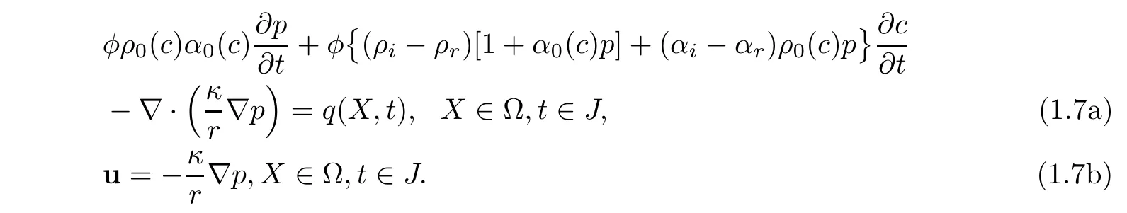
The mathematical model is defined by a nonlinear coupled system with initial-boundary conditions[1–8]:
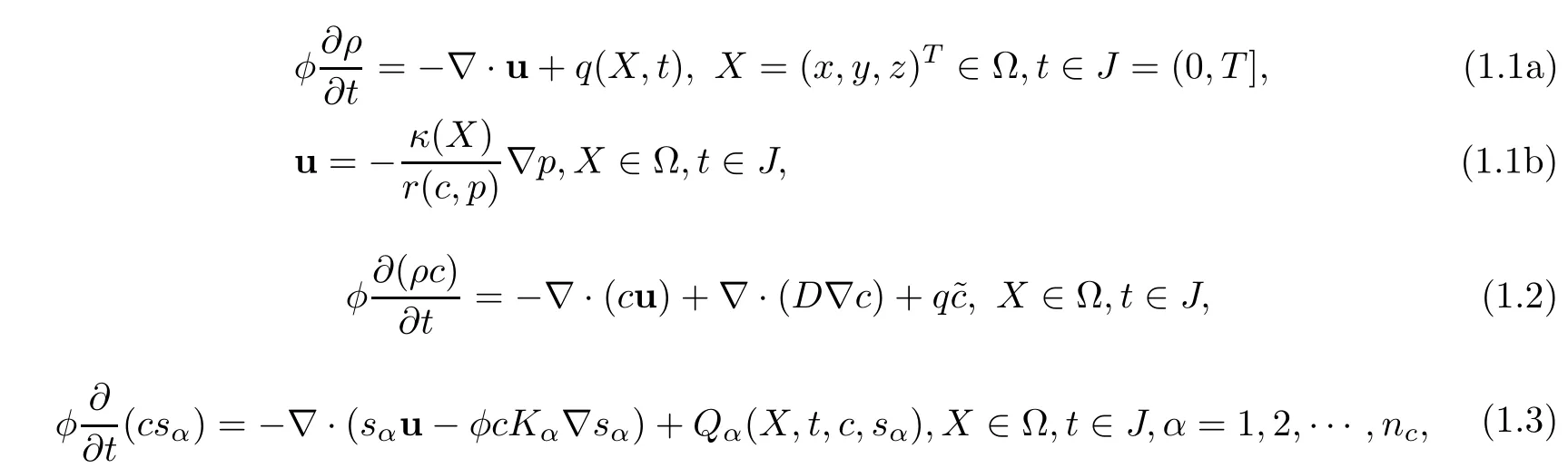
where φ = φ(X)is the porosity.ρ,the density,is defined by a function of the pressure p(X,t)and the concentration c(X,t),

where ρ0is the density of normal state,a linear function of two positive constants,the density of original flow ρrand the density of injected fluid ρi,

The coefficient of compressibility is defined by a linear function of αrand αi,the compressibility of original fluid and the compressibility of injected fluid,

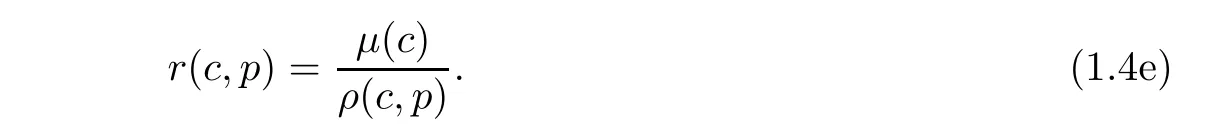
The viscosityµ=µ(c)is defined by
whereµrand µiare positive constants corresponding to original fluid and injected fluid.
The motion viscosity r is defined by the quotient of the fluid viscosity and the density,
u=u(X,t)denotes Darcy velocity of the fluid.κ= κ(X)is the permeability.Ω denotes a bounded domain of R3with the boundary ∂Ω.q is the production and D=D(X)is the diffusion coefficient determined by Fick’s Law.˜c(X,t)is equal to 1 at injection well(q>0)and is c(X,t)at production well(q < 0).The saturations of different components are denoted by sα(X,t)(α =1,2,···,nc),including different chemical agents such as the polymer,surfactant,alkali,and kinds of ions.ncis the number of components and Qαis the source sink term.
We assume that no flow of fluid moves across the boundary(Impermeable boundary conditions)
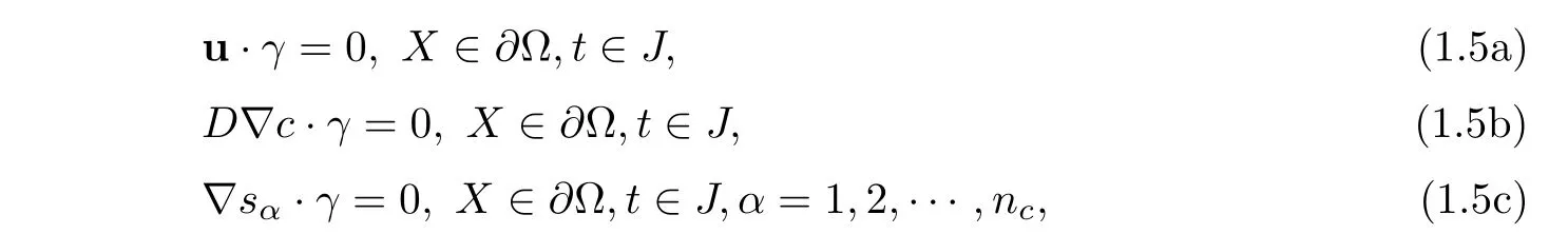
where γ is the outer normal vector to ∂Ω.
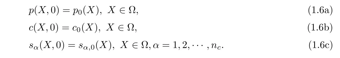
Initial conditions are listed as follows:
Using the density function(1.4),we reexpress(1.1)as follows:

For simplicity,(1.3)is stated as follows,

For incompressible two-phase displacement problem,Douglas,Ewing,Russell,Wheeler,and Yuan give a series of researches[9–12].It is well known as in numerical experiments and numerical analysis that standard finite element method in solving the convection-dominated diffusion equations does produce strong numerical dispersion and nonphysical oscillation.A variety of new numerical techniques are put forward to overcome these faults,such as characteristic finite difference[13],characteristic finite element[14],upstream-weighted finite difference[15],high-order Godunov scheme[16],streamline diffusion method[17],least squares mixed finite element[18],the modified method of characteristic finite element method(MMOC-Galerkin)[19],and the Eulerian-Lagrangian localized adjoint method(ELLAM)[20].All the above numerical methods are developed from standard finite element and finite difference,while they have some distinct disadvantages.Upstream weighted difference method tends to introduce an excess of numerical dispersion into the solution near the sharp fronts.High-order Godunov scheme requires an additional CTL restriction with respect to time step.Streamline diffusion method and least squares mixed finite element method reduce numerical dispersion but add some numerical work to define and handle artificial streamline directions.ELLAM can conserve mass locally but need large-scale computation to evaluate the resulting integrals.MMOC-Galerkin,an implicit scheme,can adopt large time step,simulate the solution at the fronts of flow stably,and avoid numerical dispersion well.While the implicit scheme is not conservative because test function is not constant.An effective method,the method of mixed finite element,is introduced to get both numerical solutions and their adjoint function of fluid mechanics with high order of accuracy.Theoretical analysis and application are discussed sufficiently in[21–23].To structure a more precise numerical scheme for convection-diffusion problem,Arbogast and Wheeler present a type of locally conservative characteristic mixed element in the timespace variation form for a convection dominated diffusion equation in[24],where the convection term is treated similarly to MMOC-Galerkin method and the diffusion is treated by zero-order Raviart-Thomas-Nedekc mixed finite element.Test function is taken by the constant function,so the scheme is locally conservative on every element.Using the postprocessing technique,Arbogast and Wheeler derive error estimates of 3/2 order.While many mapping integrals of test functions are introduced and they make the computation more complicated and difficult.
The compressibility is an important factor in modern numerical simulation of energy and environmental sciences especial of chemical oil recovery to avoid numerical distortion[1–6].Douglas and Yuan discuss a series of work for two-phase compressible displacement problem[2,25],such as the method of characteristic finite element[26,27],characteristic finite difference[28],and fractional step difference[28,29].Then,we improve and develop the work of Arbogast and Wheeler greatly[24,30,31],and present a type of mixed finite element-characteristic mixed finite element method.From experimental tests,we find that this method can shorten computational work greatly and the method is applicable and effective[30,31].While we only obtain the convergence rate of first order and can not generalize this application to solve three-dimensional problems.
Finite volume element method has the simplicity of finite differences and the high accuracy of finite element method,and has local conservation of mass[32,33],so it becomes an efficient numerical method for solving partial differential equations.In[21–23],mixed finite element can obtain both the pressure and Darcy velocity simultaneously and the accuracy is improved by one order.A mixed finite volume element method is discussed in[34,35]by combining the method of finite volume element and the method of mixed element.Its computational efficiency is testified experimentally in[36,37].Convergence analysis is mainly stated for elliptic problems in[38–40],and the general theoretical frame is established.Rui and Pan use this method to discuss numerical computation for hypotonic oil-gas flow problems in[41,42].For numerical simulation of chemical oil recovery,Ewing and Yuan have primary work for several numerical methods and give actual applications,such as upwind difference[43]and characteristic finite difference[44].While these methods do not have the conservative law of mass.Based on the above work,a type of mixed volume element-characteristic fractional step difference method is put forward to simulate three-dimensional compressible chemical oil recovery in this article.The pressure and Darcy velocity are computed simultaneously by a conservative mixed volume element method and the computational accuracy of Darcy velocity is improved one order.The concentration is treated by another conservative characteristic mixed finite volume element method,where the convection is approximated along the characteristics and the diffusion is discretized by the method of mixed volume element.The characteristics not only has high stability at sharp fronts and eliminates numerical dispersion,but also has small time truncation error.In actual computations,large time step can be used while computational efficiency is improved without accuracy loss.We adopt mixed finite volume element to treat the diffusion and obtain unknown concentration and adjoint vector simultaneously.Because piecewise defined constants are taken as test functions,so the scheme is locally conservative.Applying priori estimates theory and special techniques of differential equations,we obtain optimal order estimates in L2norm,superior to 3/2-order result of Arbogast and Wheeler without postprocessing[24].The saturations of different components,whose computational work is the largest,are treated by characteristic fractional step differences.The whole computation is changed into three one-dimensional problems computed by the algorithm of speedup,then the computational work is shortened greatly[2,45].In this article,numerical experiments are given for a three-dimensional system of elliptic-convection-diffusion equations,then these data show that this method is effective and support theoretical result.Moreover,this method gives an efficient tool to solve the well-known problem successfully[1–6,24,46].
Common notations and norms of Sobolev space are adopted in this article.The regularity assumptions of(1.1)–(1.9)are stated as follows:
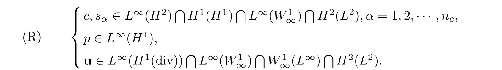
Suppose that the coefficients of(1.1)–(1.9)satisfy the following positive definite conditions

where a∗,a∗,φ∗,φ∗,D∗,and D∗are positive constants.
In this article,assume that the problem of(1.1)–(1.9)is Ω-periodic to discuss theoretical analysis[2,9–12],that is to say,all the functions are Ω-periodic.This periodicity assumption is reasonable in physics,because mirror re flection is used according to(1.5).Furthermore,the boundary conditions can be omitted because they give less effect to the interior flow in common numerical simulation of oil reservoir[9–12].
In the following discussion,the symbols K and ε denote a generic positive constant and a generic small positive number,respectively.They have different definitions at different places.
2 Notations and Preparations
Three different partitions are constructed to define the method of mixed volume elementcharacteristic fractional step differences.The large-step partition is nonuniform for the pressure and Darcy velocity.The mid-step nonuniform partition is defined for the concentration.The small-step uniform partition is defined for the concentrations of different components.The first two partitions are considered.
For the simplicity of discussing three-dimensional problem,take Ω={[0,1]}3with the boundary∂Ω.Define
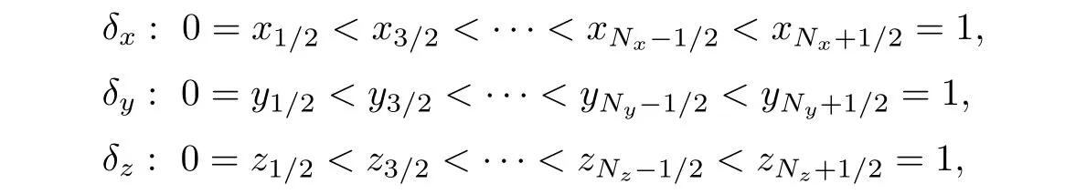
then partition Ω by δx× δy× δz.For i=1,2,···,Nx;j=1,2,···,Ny;k=1,2,···,Nz,define the following notations,The partition is regular,if there exist two positive constants α1and α2such that

Here, α1and α2are positive constants dependent on the partition of Ω, δx× δy× δz.The simplified partition of Nx=4,Ny=3,and Nz=3 is illustrated in Figure 1.Define an approximation function space bywhere pd(Ωi)denotes a space consisting of polynomial functions of degree at most d constricted onThe function f may be discontinuous on[0,1]as l= −1.The spacesandare defined similarly.Let
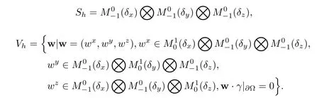
For a grid function v(x,y,z),let vijk,vi+1/2,jk,vi,j+1/2,k,and vij,k+1/2denote its values at(xi,yj,zk),(xi+1/2,yj,zk),(xi,yj+1/2,zk),and(xi,yj,zk+1/2),respectively.
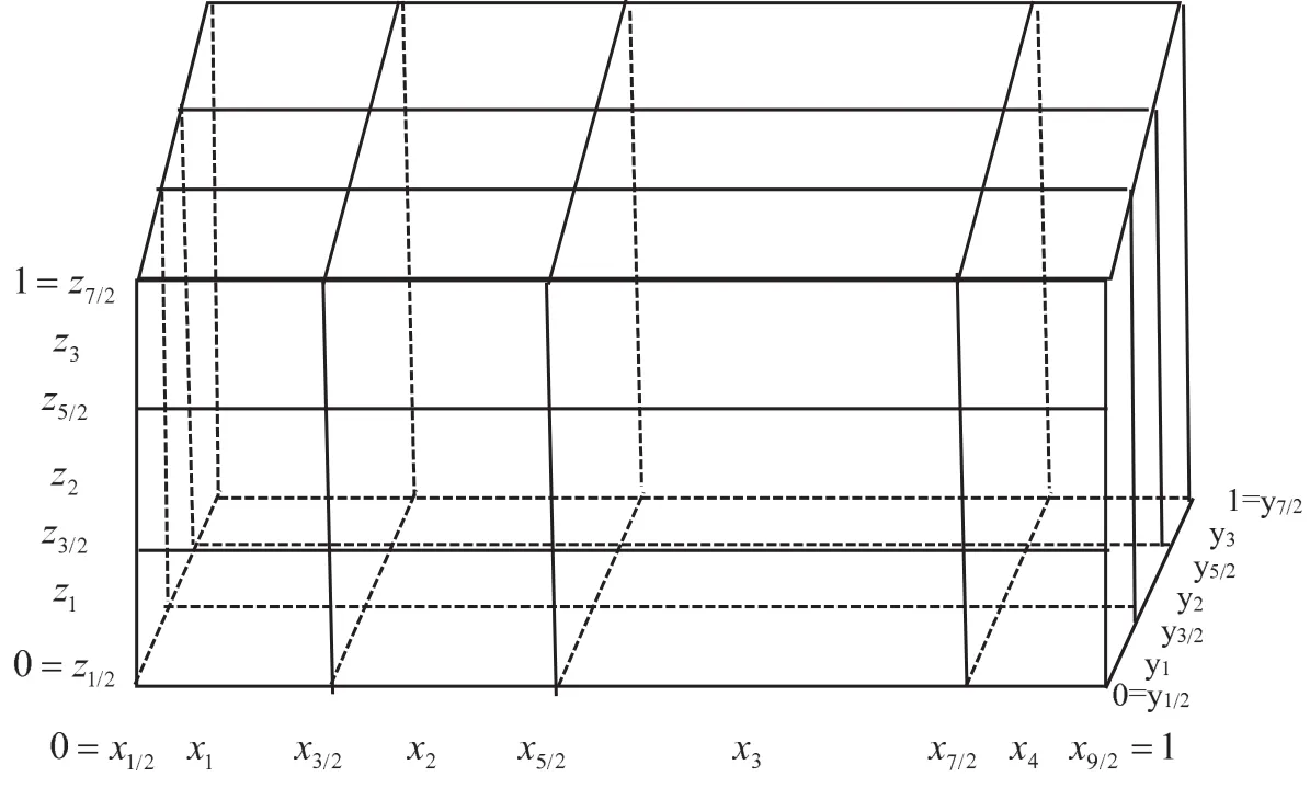
Figure 1 Nonuniform partition
Define inner products and norms by
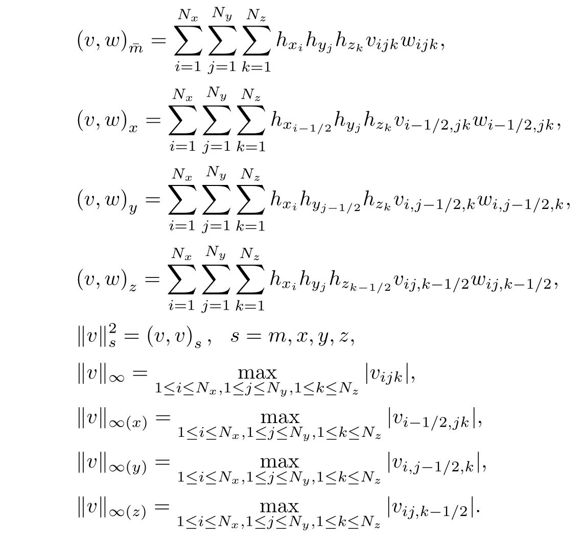
For a vector function w=(wx,wy,wz)T,let


Introduce difference operators and other notations as follows:
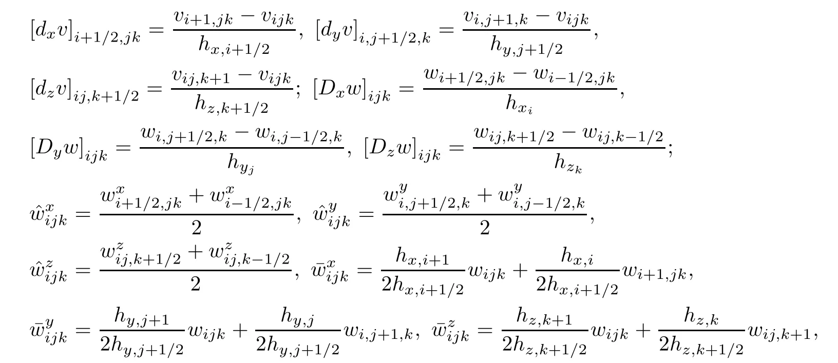
Using the above notations,we give four preparations for convergence analysis.
Lemma 2.1For v∈Shand w∈Vh,we have

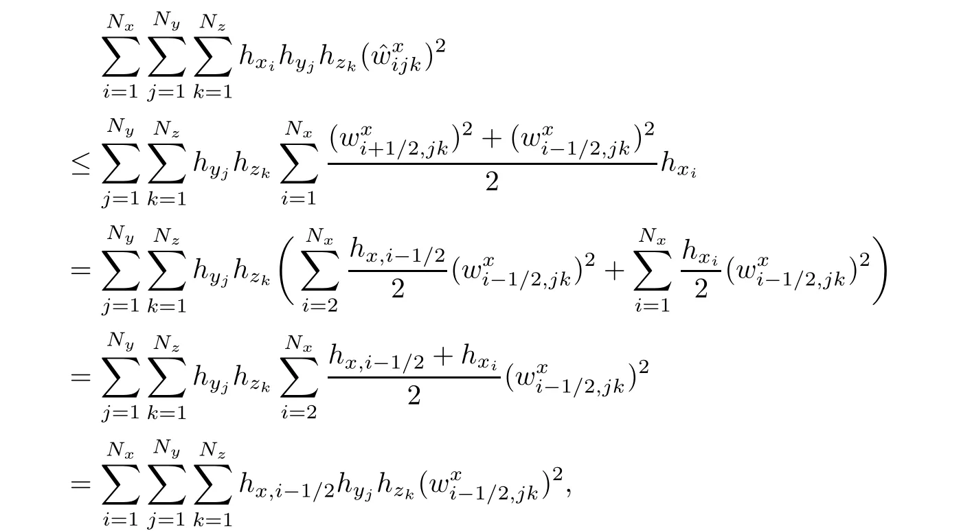
Lemma 2.2For w∈Vh,we have

ProofIt is adequate to prove that‖ˆwx‖¯m≤‖wx‖x,‖ˆwy‖¯m≤‖wy‖y,and‖ˆwz‖¯m≤‖wz‖z.From the fact that
Lemma 2.3For q∈Sh,we have

where M is a constant independent of q and h.
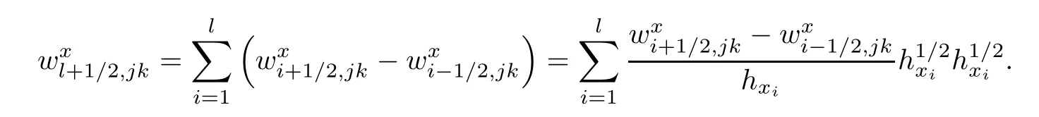
Lemma 2.4For w∈Vh,there hold

ProofIt is adequate to proveand the other terms are proved similarly.Note that
By Cauchy inequality,we have
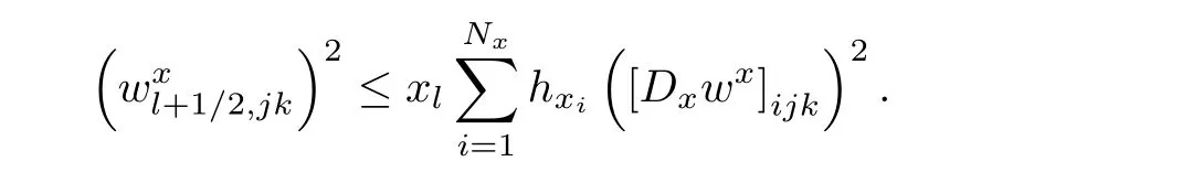
Multiplying both sides by hx,i+1/2hyjhzk,and making the summation,we have
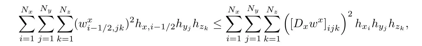
then we complete the proof.
The mid-step partition is defined by refining the large-step partition of Ω={[0,1]}3uniformly,where the step is assigned by 1/2 or 1/4 times the large step,and hc=hp/l for l=2 or l=4.Other notations are defined above.
The small-step partition of Ω={[0,1]}3is defined uniformly,
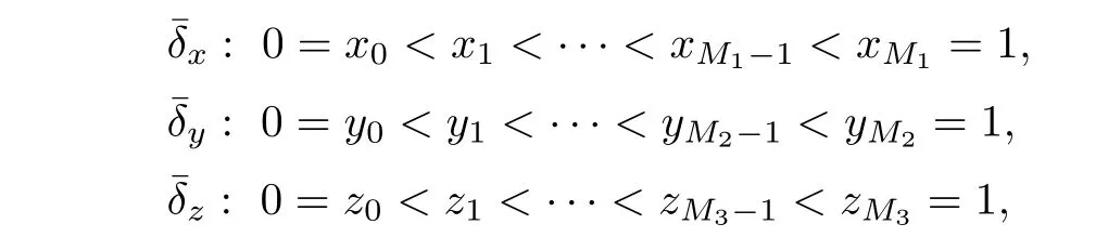
where M1,M2,and M3are positive constants.Three steps along different directions and nodes are denoted byD(Xi−1,jk)],and define Di,j+1/2,k,Di,j−1/2,k,Dij,k+1/2,Dij,k−1/2similarly.Define

3 The Procedures of Mixed Volume Element-Characteristic Mixed Volume Element Method
3.1 The procedures

To apply mixed volume element method,we rewrite the flow equation(1.7)in the following standard form

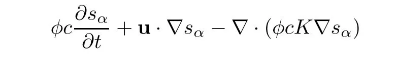
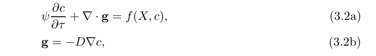
For the concentration(1.8),noting that the flow transports along the characteristics,so we use the method of characteristics to approximate the first-order hyperbolic term and construct a computational algorithm of strong stability and of high order accuracy with large time steps.To argue the diffusion term using mixed volume element method,we reexpress(1.8)as follows:
The characteristic derivative of(3.2a)is approximated by the backward difference quotient,

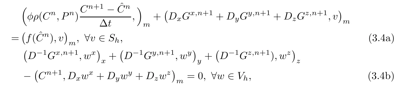
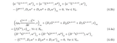
The procedures of mixed volume element of(3.1)are defined by

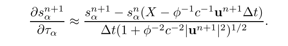
Because the saturations of(1.9)are computed with high order of accuracy,so the computational work is quite large.The method of characteristics is applied to treat hyperbolic term,and it has some advantages of stability and accuracy.LetWe state(1.9)as follows:


The characteristic derivative in(3.6)is treated by using the backward difference quotient operator
The procedures of characteristic fractional step difference of(3.6)are stated as follows:

Initial approximations are listed as follows:

Numerical solutions are computed by the method of mixed volume element-characteristic mixed volume element below.From(1.6)and elliptic projections of mixed volume element,we getandthen defineandUsing scheme(3.4)and the method of conjugate gradient obtains{C1,G1}.Similarly,we obtain{U1,P1}from(3.5).Next,we use the parallel scheme(3.8a)–(3.8c)and the algorithm of speedup to get the values of transient layersthen to get the values atThe computation at the first time level is completed.After the same computation,we haveone by one from the procedures(3.4),(3.5),and(3.8a)–(3.8c).Finally,we can obtain all the numerical solutions after repeated computations,and see that the solutions exist and are unique from the condition(C).
3.2 Local conservation of mass
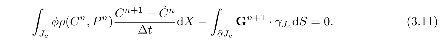
Suppose that the problem(3.1)–(3.2)has no source or sink,that is,q ≡ 0,and suppose that the boundary condition is impermeable.Then,for simplicity,suppose that the first two partitions are the same(that is l=1)on each element Jc∈ Ω,Jc= Ωijk=[xi−1/2,xi+1/2]×[yj−1/2,yj+1/2]× [zk−1/2,zk+1/2].The local conservation of mass is interpreted as follows for the concentration equation

where Jcis an element of mid-step partition of Ω,and γJcdenotes the outer normal vector to the boundary∂Jc.Discrete formulation of local conservation is stated in the following theorem for(3.4a).
Theorem 3.1If q≡0,then on each element Jc∈Ω,it holds that for the scheme(3.4a),
ProofFor v∈Sh,letthen we rewrite(3.4a)as follows

Using the notations of Section 2,
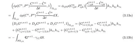
Substituting(3.13)into(3.12),then we complete the proof.
Then,the conservation of mass on the whole domain is derived as follows.
Theorem 3.2Suppose that q≡0 and the boundary condition is impermeable.Then,the whole conservation of mass of(3.4a)holds,

ProofSumming(3.11)on all the elements,we have

3.3 Auxiliary elliptic projections
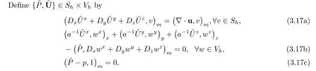
In this subsection,we define the elliptic projections to determine initial approximations(3.9)and to show convergence analysis in the next section.Define{˜C,˜G}∈Sh×Vhby the following equations:
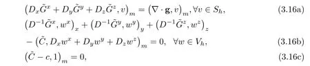
where g=−D∇c.
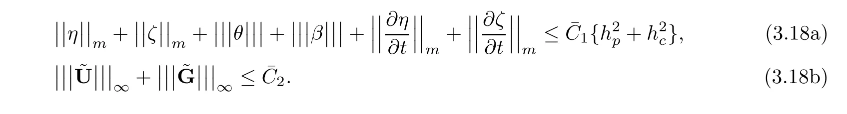
Lemma 3.3If the coefficients and exact solutions of(1.1)-(1.6)satisfy(C)and(R),then there exist two positive constantsindependent of h,Δt such that
4 Convergence Analysis
In this section,we give convergence argument for a model problem.In(1.7)and(1.8),some coefficients are simplified as follows:ρi≈ ρr,αi≈ αr,ρ(c,p)≈ ρ0,µ(c)≈ µ0,a(c,p)=which is reasonable for ”slight-compressibility”low seepage problem[8,47].Then,
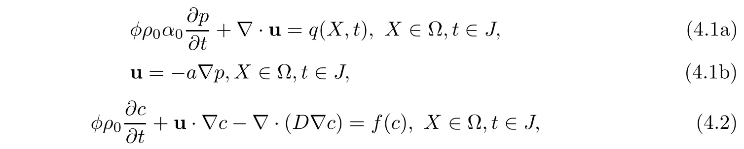
where ρ0,α0,µ0are positive constants.Therefore,the procedures of(1.7)and(1.8)are simplified as follows:

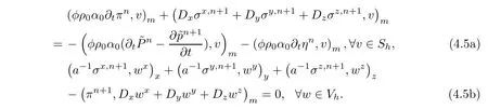
Error functions π and σ are considered first.Subtracting(3.17a)(t=tn+1)and(3.17b)(t=tn+1)from(4.3a)and(4.3b),respectively
Take v= ∂tπnin(4.5a).Make the difference of(4.5b)at tn+1and at tn,divide the difference by Δt,and take w= σn+1.Summing the two resulting formulations,and noting that for A≥0,

then we have
From(C)and Lemma 3.3,we have
Using(4.7)to consider the right-hand terms of(4.6),we obtain

Multiplying the both sides of(4.8)by Δt,summing them on t(0≤ n ≤ L),and noting that σ0=0,we have

Error function of the concentration is discussed.Subtracting(3.16a),(3.16b)at t=tn+1respectively from(4.4a),(4.4b),and taking v= ξn+1,w= αn+1,then

Consider the sum of(4.10a)and(4.10b),
Using(4.2)t=tn+1,we have

The left-hand terms of(4.12)are estimated by usingand the righthand terms are denoted by T1,T2,···,T8,

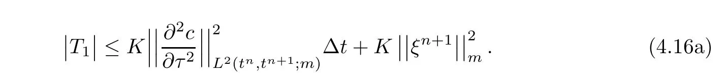
T1is considered first.Noting thatwe have

Multiplying the both sides of(4.14)by ψn+1and estimating it in m-norm,we obtain

Therefore,
Applying Lemma 3.3,we estimate T2 and T3by

T4,T5,and T6are estimated from the following statement.Let f be defined on Ω,denoting three functions,andand let Z denote the normal vector of Un+1−un+1.Then,
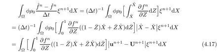
then we get three arguments from(4.17):
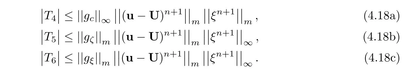
From Lemma 3.3 and(4.9),

As gˆc(X)is a mean value of partial derivative of,so it can be estimated by.From(4.18a),


and give a constraint condition

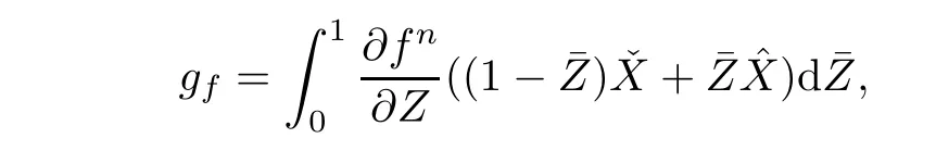
The function gfis bounded by
Define a transformation

It follows from(4.21)and(4.22)that

Then,gfis bounded by

T5is argued using(4.19),Lemma 3.3,and Sobolev embedding theorem[48],
It follows obviously from(4.19)thatand it shows thatin(4.8).Similar to[11],we have

By negative norm estimates,T7and T8are bounded by
Applying(4.8),(4.16),(4.18),(4.26),and(4.27)for the both sides of(4.12),we have
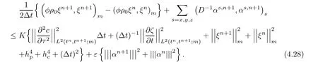
Multiplying the both sides of(4.28)by 2Δt,summing them on t(0≤ n≤ L),noting that ξ0=0,and using the Gronwall’lemma,we get
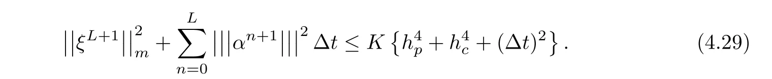
It remains to testify the induction hypothesis(4.21).It is true for n=0 obviously from ξ0=0.Assume that(4.21)holds for 1≤n≤L.From(4.29)and(4.22),we have

Then,the induction hypothesis is proved for n=L.
Error functions of component saturations are considered.LetFor a model problem,(1.9)turns into

Suppose that c(X,t)is known and regular.Cancelling the values of transition layersfrom(3.8a),(3.8b),and(3.8c),we have the following equivalent formulation
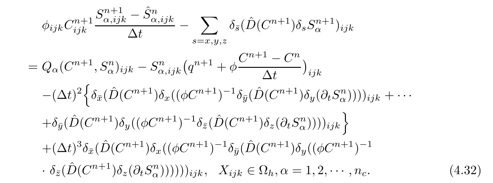
Making the difference of(4.31)(t=tn+1)and(4.32)(t=tn+1),
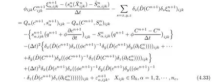
Considering(4.9),(3.7),and(4.33)together,we get
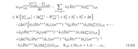
Multiplying the both sides of(4.34)by,summing by parts and giving an inner product form,we obtain

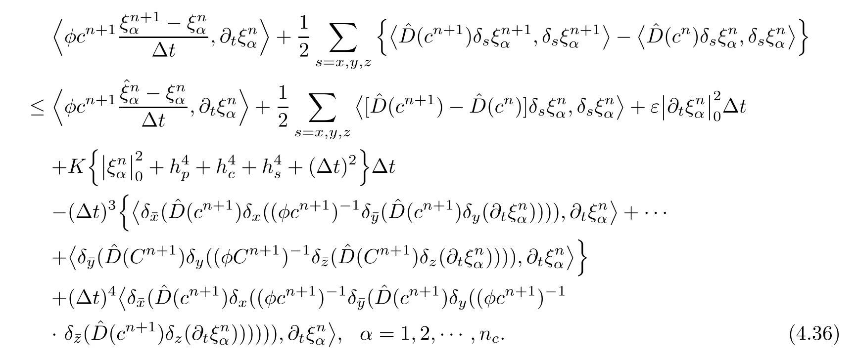
The first term on the right-hand side of(4.36)is considered.Considering the fact that

(4.22),and(4.9)together,we have

where Ωhdenotes a small-step partition of Ω,
The second term on the right-hand side of(4.36)is estimated by

The fifth term on the right-hand side of(4.36)is discussed.Note that

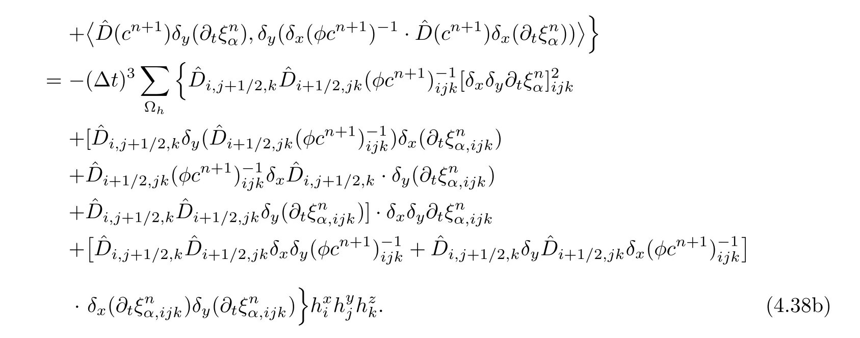
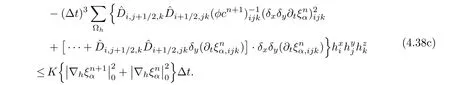
Because of the regularity of φc,the last term of(4.38b)is treated by
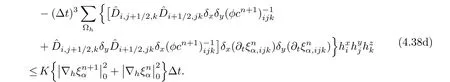
The other two parts of the fifth term are discussed similarly.Then,
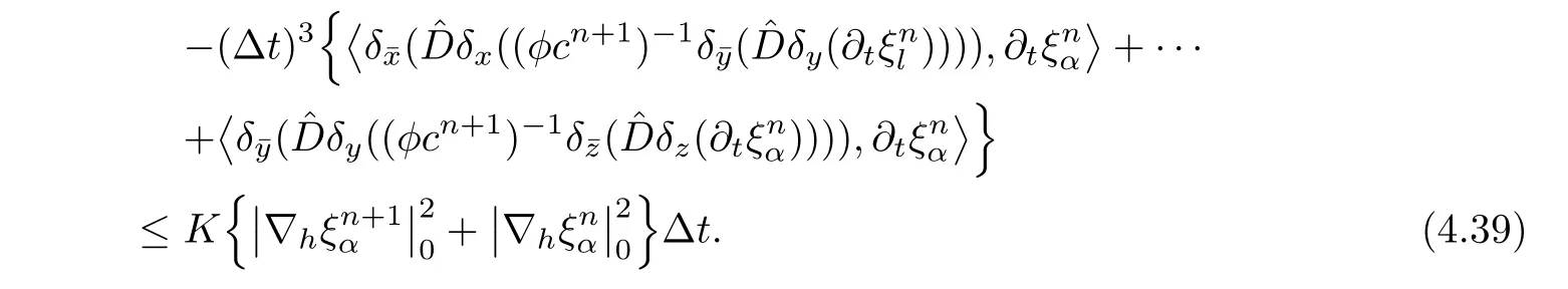
For the last term on the right-hand side of(4.36),we cancelsimilarly by using Cauchy inequality,and get
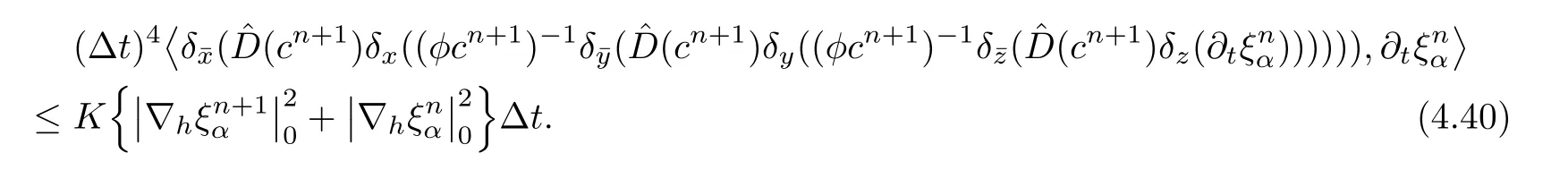
Considering(4.37),(4.39),(4.40),and(4.36),we obtain

Summing the resulting estimate(4.41)on α(1≤α≤nc),then summing them on t(0≤n≤L),and noting that=0,α=1,2,···,nc,we have


Collecting(4.9),(4.29),(4.43),and Lemma 3.3,we conclude the following statement.
Theorem 4.1Suppose that exact solutions of(4.1)–(4.2)are regular(R)and coefficients are positive definite(C).Adopt the procedures(4.3)and(4.4)to get numerical solutions,then use the schemes(3.8a),(3.8b)and(3.8c)to solve equation(4.31).The constraint condition(4.22)holds.Then,

5 Numerical Examples
We assume that Darcy velocity u is given,and adopt the characteristics-mixed volume element scheme to approximate a convection-diffusion equation first,

where Ω =(0,1)× (0,1)× (0,1)and ν is the outer normal vector to ∂Ω.Darcy velocity u=(u1,u2,u3)Tis defined as follows:
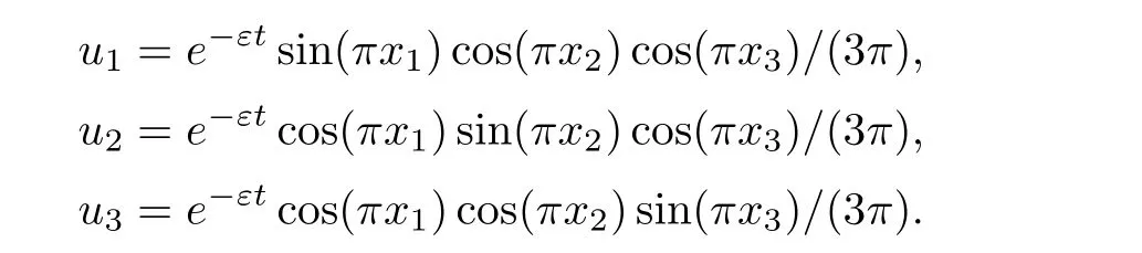
f and c0are defined suitably such that exact solution is c=e−εtcos(πx1)cos(πx2)cos(πx3)/(3π).
The concentration and its adjoint function of(5.1)are approximated by the characteristicsmixed volume element.Take Δt=0.001,t=1.0,and give numerical results for different cases ε=1,10−3,10−8.Error data ofc−Ch,g−Ghare shown in Table 1 and Table 2,where·hdenotes discrete l2norm.Errors become small as step decreases,and the convergence rate is about second order no less than first order.At x3=0.28152,the approximations of c−C and g − G for ε=10−3are shown in Figures 2–5.
Table 1 Error data ofc−Chfor Example 1
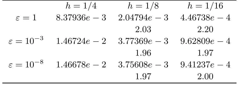
Table 1 Error data ofc−Chfor Example 1
?
Table 2 Error data ofg−Ghfor Example 1

Table 2 Error data ofg−Ghfor Example 1
?
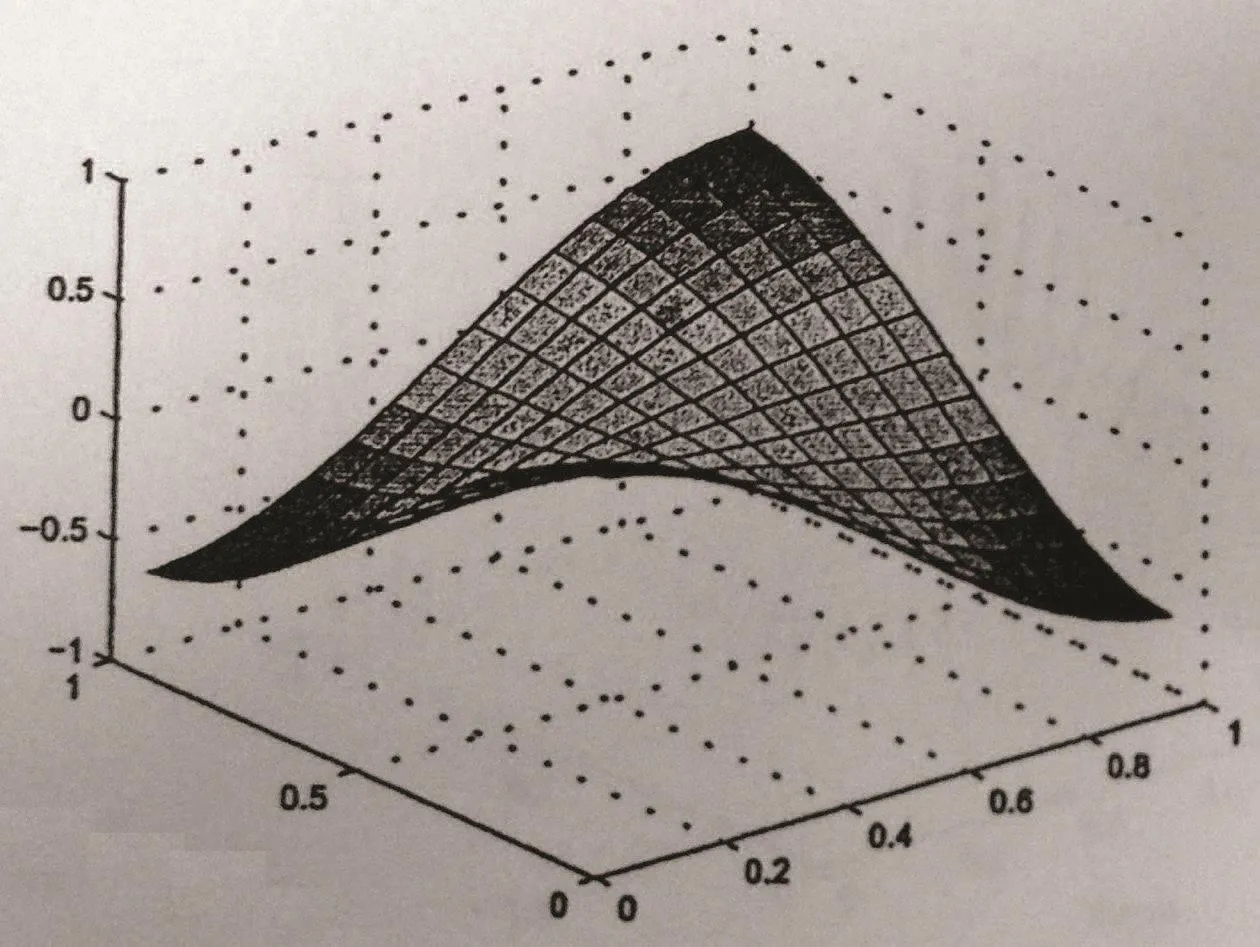
Figure 2 Section graph of c at t=1,h=1/16

Figure 3 Section graph of C at t=1,h=1/16
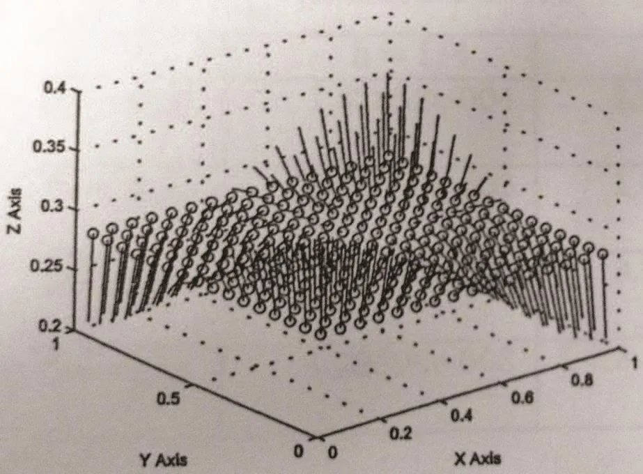
Figure 4 Arrow graph of g at t=1,h=1/16

Figure 5 Arrow graph of G at t=1,h=1/16
From Table 1,Table 2,and Figures 2–5,we can conclude that this scheme is stable and efficient to simulate the functions c and g,and it is effective for small ε.
We use the scheme of mixed volume element-characteristic mixed finite element to solve another elliptic-convection-diffusion problem,
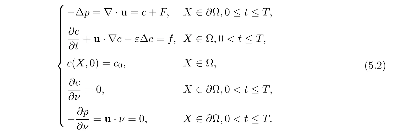
Ω =(0,1)×(0,1)×(0,1)and ν is the outer normal vector to the boundary ∂Ω.F,f,and c0are defined properly such that exact solutions are
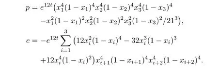
where x4=x1,x5=x2.We use the scheme of mixed volume element to approximate the first equation of(5.2),and use the characteristics-mixed finite element to solve the second equation.Numerical data are shown for ε=10−3in Table 3 and Figures 6–13.
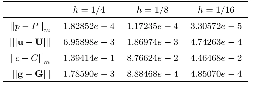
Table 3 Error data for Example 2
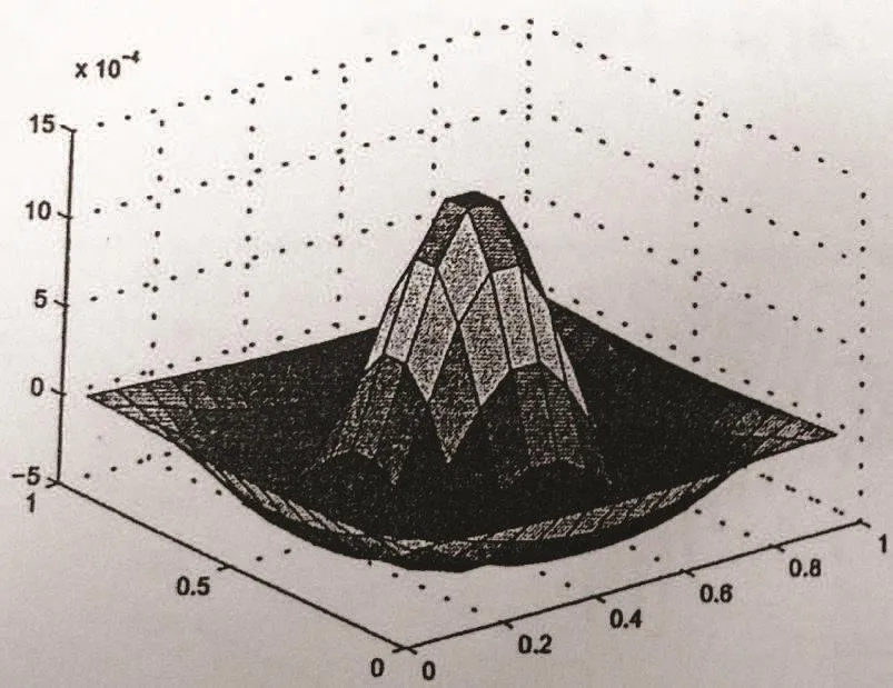
Figure 6 Section graph of p at t=1,h=1/16

Figure 7 Section graph of P at t=1,h=1/16
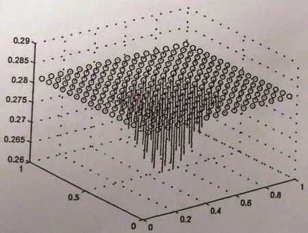
Figure 8 Arrow graph of u at t=1,h=1/16
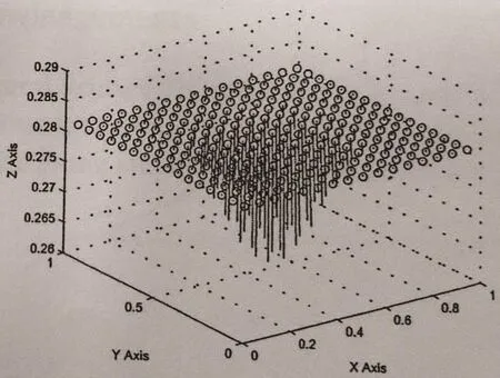
Figure 9 Arrow graph of U at t=1,h=1/16

Figure 10 Section graph of c at t=1,h=1/16
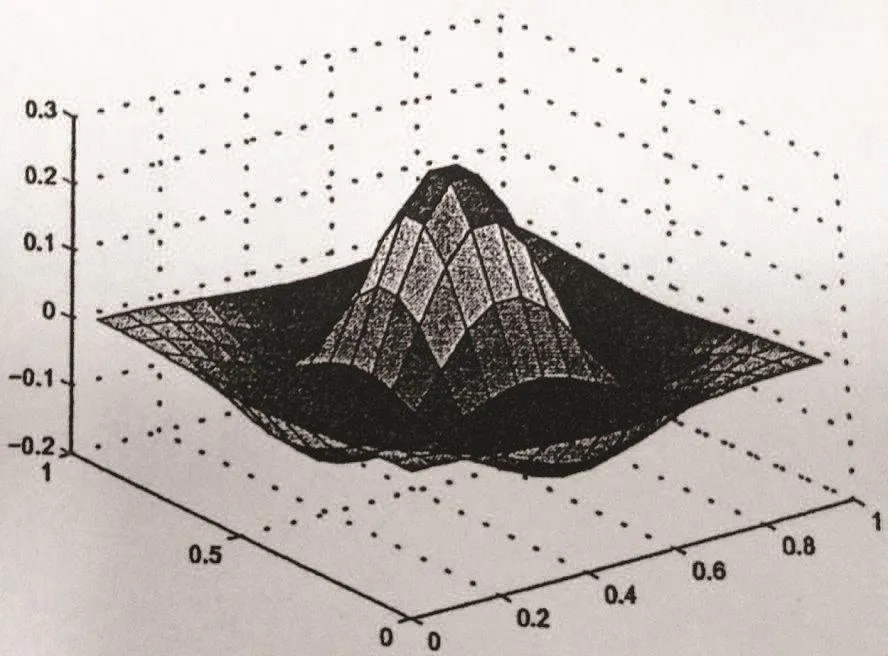
Figure 11 Section graph of C at t=1,h=1/16
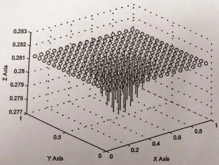
Figure 12 Arrow graph of g at t=1,h=1/16
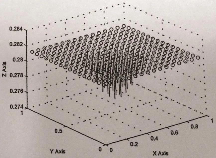
Figure 13 Arrow graph of G at t=1,h=1/16
From Table 3 and Figures 6–13,we find that this numerical method is effective in solving convection-diffusion problems.
6 Conclusions and Discussions
Numerical simulation of three-dimensional chemical oil recovery in porous media is discussed in this article.A composite method of mixed finite volume element-characteristic mixed volume element is presented and its convergence analysis is shown.In Section 1,mathematical model is stated,and physical background and some related international study are introduced.In Section 2,some notations and preparations are introduced,and three different partitions(large-step,mid-step and small-step)are defined for approximating three unknown functions.In Section 3,the authors put forward the method of mixed volume element-characteristic mixed volume element.The flow equation is treated by a conservative mixed volume element scheme and the accuracy of Darcy velocity is improved by one order.The method of characteristic mixed volume element is applied to solve the concentration,where the convection term is treated by the method of characteristics and the diffusion term is approximated by the method of mixed volume element.The composite scheme improves computational stability and accuracy greatly and it has the nature of conservation most important in numerical simulation of underground seepage mechanics.The method of characteristic fractional step difference is used to solve the saturation equations of different components whose computational work is the largest.By dividing the problem into three one-dimensional subproblems and using the algorithm of speedup,the computational work is shorten greatly and the computational efficiency is improved.In Section 4,we show convergence analysis using the priori estimates of differential equations and special techniques to derive second order error estimates in l2norm.It is most important to improve the famous convergence result of 3/2-order of Arbogast and Wheeler.In Section 5,two numerical examples are illustrated to support theoretical analysis and numerical data show that the method is feasible and efficient in actual applications especially in waste disposal problem of environmental science.
In this article,several interesting conclusions are stated as follows:
(I)The method has physical nature of conservation,and it is most important in numerical simulation of underground seepage mechanics especially in chemical oil recovery.
(II)The method is a composite combination of mixed volume element,the characteristics,and fractional step difference,so it has strong stability and high accuracy.Therefore,it is more useful especially in simulating large-scaled engineering problems on three-dimensional complicated region.
(III) The method increases convergence rate of 3/2-order of Arbogast and Wheeler to second order,and it gives a powerful tool to solve the problem better[1–6,24,46].
AcknowledgementsThe authors express their deep appreciation to Prof.J.Douglas Jr,Prof.R.E.Ewing,and Prof.L.S.Jiang for their many helpful suggestions in the series research on numerical simulation of oil reservoir.
[1]Ewing R E,Yuan Y R,Li G.Finite element for chemical- flooding simulation.Proceeding of the 7th International conference finite element method in flow problems.The University of Alabama in Huntsville,Huntsville,Alabama:UAHDRESS,1989:1264–1271
[2]Yuan Y R.Theory and application of numerical simulation of energy sources.Beijing:Science Press,2013:257–304
[3]Yuan Y R,Yang D P,Qi L Q,et al.Research on algorithms of applied software of the polymer.Qinlin Gang,Proceedings on chemical flooding.Beijing:Petroleum Industry Press,1998:246–253
[4]Institute of Mathematics,Shandong University,Exploration Institute of Daqing Petroleum Administration Bureau.Research and application of the polymer flooding software(summary of”Eighth-Five” national key science and technology program,Grant No.85-203-01-08),1995.10
[5]Institute of Mathematics,Shandong University,Exploration and development of Daqing Petroleum Corporation.Modification of solving mathematical models of the polymer and improvement of reservoir description(DQYT-1201002-2006-JS-9765).2006.10
[6]Institute of Mathematics,Shandong University,Shengli Oilfield Branch,China Petroleum&Chemical.Research on key technology of high temperature and high salinity chemical agent displacement(2008ZX05011-004),83-106.2011.3
[7]Bird R B,Lightfoot W E,Stewart E N.Transport Phenomenon.New York:John Wiley and Sons,1960
[8]Ewing R E.The Mathematics of Reservior Simulation.Philadelphia:SIAM,1983
[9]Douglas J Jr.Finite difference method for two-phase in compressible flwo in porous media.SIAM J Numer Anal,1983,20(4):681–696
[10]Russell T F.Time stepping along characteristics with incomplete interaction for a Galerkin approximation of miscible displacement in porous media.SLAM J Numer Anal,1985,22(5):970–1013
[11]Ewing R E,Russell T F,Wheeler M F.Convergence analysis of an approximation of miscible displacement in porous media by mixed finite elements and a modified method of characteristics.Comput Methods Appl Mech Engrg,1984,47(1/2):73–92
[12]Douglas Jr J,Yuan Y R.Numerical simulation of immiscible flow in porous media based on combining the method of characteristics with mixed finite element procedure.Numerical Simulation in Oil Rewvery.New York:Springer-Berlag,1986:119–132
[13]Yuan Y R.Characteristic finite difference methods for positive semidefinite problem of two phase miscible flow in porous media.J Systems Sci Math Sci,1999,12(4):299–306
[14]Yuan Y R.Characteristic finite element methods for positive semidefinite problem of two phase miscible flow in three dimensions.Chin Sci Bull,1996,41(22):2027–2032
[15]Todd M R,O’Dell P M,Hirasaki G J.Methods for increased accuracy in numerical reservoir simulators.Soc Petrol Engry J,1972,12(6):521–530
[16]Bell J B,Dawson C N,Shubin G R.An unsplit high-order Godunov scheme for scalar conservation laws in two dimensions.J Comput Phys,1988,74(1):1–24
[17]Johnson C.Streamline diffusion methods for problems in fluid mechanics//Finite Element in Fluids VI.New York:Wiley,1986
[18]Yang D P.Analysis of least-squares mixed finite element methods for nonlinear nonstationary convectiondiffusion problems.Math Comp,2000,69(231):929–963
[19]Dawson C N,Russell T F,Wheeler M F.Some improved error estimates for the modified method of characteristics.SIAM J Numer Anal,1989,26(6):1487–1512
[20]Cella M A,Russell T F,Herrera I,Ewing R E.An Eulerian-Lagrangian localized adjoint method for the advection-diffusion equations.Adv Water Resour,1990,13(4):187–206
[21]Raviart P A,Thomas J M.A mixed finite element method for second order elliptic problems//Mathematical Aspects of the Finite Element Method.Lecture Notes in Mathematics,606.Berlin:Springer-Verlag,1977
[22]Douglas J Jr,Ewing R E,Wheeler M F.Approximation of the pressure by a mixed method in the simulation of miscible displacement.RAIRO Anal Numer,1983,17(1):17–33
[23]Douglas J Jr,Ewing R E,Wheeler M F.A time-discretization procedure for a mixed finite element approximation of miscible displacement in porous media.RAIRO Anal Numer,1983,17(3):249–265
[24]Arbogast T,Wheeler M F.A charcteristics-mixed finite element methods for advection-dominated transport problems.SIAMJ Numer Anal,1995,32(2):404–424
[25]Douglas J Jr,Roberts J E.Numerical methods for a model for compressible miscible displacement in porous media.Math Comp,1983,41(164):441–459
[26]Yuan Y R.The characteristic finite element alternating direction method with moving meshes for nonlinear convection-dominated diffusion problems.Numer Meth Part D E,2006,22(3):661–679
[27]Yuan Y R.The modified method of characteristics with finite element operator-splitting procedures for compressible multi-component displacement problem.J Syst Sci Complexj,2003,16(1):30–45
[28]Yuan Y R.The characteristic finite difference fractional steps method for compressible two-phase displacement problem(in Chinese).Sci Sin Math,1999,42(1):48–57
[29]Yuan Y R.The upwind finite difference fractional steps methods for two-phase compressible flow in porous media.Numer Meth Part D E,2003,19(1):67–88
[30]Sun T J,Yuan Y R.An approximation of incompressible miscible displacement in porous media by mixed finite element method and characteristics-mixed finite element method.J Comput Appl Math,2009,228(1):391–411
[31]Sun T J,Yuan Y R.Mixed finite method and characteristics-mixed finite element method for a slightly compressible miscible displacement problem in porous media.Math Comput Simulat,2015,107:24–45
[32]Cai Z.On the finite volume element method.Numer Math,1991,58(1):713–735
[33]Li R H,Chen Z Y.Generalized difference of differential equations.Changchun:Jilin University Press,1994
[34]Russell T F.Rigorous block-centered discritization on inregular grids:Improved simulation of complex reservoir systems.Project Report.Tulsa:Research Comporation,1995
[35]Weiser A,Wheeler M F.On convergence of block-centered finite difference for elliptic problems.SIAM J Numer Anal,1988,25(2):351–375
[36]Jones J E.A mixed volume method for accurate computation of fluid velocities in porous media[D/OL].Denver,Co:University of Colorado,1995
[37]Cai Z,Jones J E,Mccormilk S F,Russell T F.Control-volume mixed finite element methods.Comput Geosci,1997,1(3):289–315
[38]Chou S H,Kawk D Y,Vassileviki P.Mixed volume methods on rectangular grids for elliptic problem.SIAM J Numer Anal,2000,37(3):758–771
[39]Chou S H,Kawk D Y,Vassileviki P.Mixed volume methods for elliptic problems on trianglar grids.SIAM J Numer Anal,1998,35(5):1850–1861
[40]Chou S H,Vassileviki P.A general mixed covolume frame work for constructing conservative schemes for elliptic problems.Math Comp,1999,68(227):991–1011
[41]Rui H X,Pan H.A block-centered finite difference method for the Darcy-Forchheimer Model.SIAM J Numer Anal,2012,50(5):2612–2631
[42]Pan H,Rui H X.Mixed element method for two-dimensional Darcy-Forchheimer model.J Sci Comput,2012,52(3):563–587
[43]Yuan Y R,Cheng A J,Yang D P,Li C F.Convergence analysis of an implicit upwind difference fractional step method of three-dimensional enhanced oil recovery percolation coupled system.Sci China Math,2014,44(10):1035–1058
[44]Yuan Y R,Cheng A J,Yang D P,Li C F.Theory and application of fractional steps characteristic- finite difference method in numerical simulation of second order enhanced oil production.Acta Mathematica Scientia,2015,35B(4):1547–1565
[45]Yuan Y R.Fractional step finite difference method for multi-dimensional mathematical-physical problems.Beijing:Science Press,2015.6
[46]Shen P P,Liu M X,Tang L.Mathematical model of petroleum exploration and development.Beijing:Science Press,2002
[47]Ewing R E,Wheeler M F.Galerkin methods for miscible displacement problems with point sources and sinks-unit mobility ratis case.Proc Special Year in Numerical Anal.Lecture Notes#20.Univ Maryland,College Park,1981:151–174
[48]Nitsche J.Linear splint-funktionen and die methoden von Ritz for elliptishce randwert probleme.Arch for Rational Mech and Anal,1968,36:348–355
[49]Douglas J Jr.Simulation of miscible displacement in porous media by a modified method of characteristic procedure//Dundee.Numerical Analysis,1981.Lecture Notes in Mathematics,912.Berlin:Springer-Verlag,1982
 Acta Mathematica Scientia(English Series)2018年2期
- Acta Mathematica Scientia(English Series)的其它文章
- ON A FIXED POINT THEOREM IN 2-BANACH SPACES AND SOME OF ITS APPLICATIONS∗
- MULTIPLICITY AND CONCENTRATION BEHAVIOUR OF POSITIVE SOLUTIONS FOR SCHRÖDINGER-KIRCHHOFF TYPE EQUATIONS INVOLVING THE p-LAPLACIAN IN RN∗
- MULTIPLICITY OF SOLUTIONS OF WEIGHTED(p,q)-LAPLACIAN WITH SMALL SOURCE∗
- QUALITATIVE ANALYSIS OF A STOCHASTIC RATIO-DEPENDENT HOLLING-TANNER SYSTEM∗
- SHARP BOUNDS FOR HARDY OPERATORS ON PRODUCT SPACES∗
- CONTINUOUS FINITE ELEMENT METHODS FOR REISSNER-MINDLIN PLATE PROBLEM∗