
SOLUTIONS TO BSDES DRIVEN BY BOTH FRACTIONAL BROWNIAN MOTIONS AND THE UNDERLYING STANDARD BROWNIAN MOTIONS∗
2018-05-05 07:09YuecaiHAN韩月才
Yuecai HAN(韩月才)
Department of Mathematical Finance,School of Mathematics,Jilin University,Changchun 130012,China
E-mail:hanyc@jlu.edu.cn
Yifang SUN(孙一芳)†
Department of Probability and Mathematical Statistics,School of Mathematics,Jilin University,Changchun 130012,China
E-mail:syf15@mails.jlu.edu.cn
1 Introduction
Let(Ω,F,P)be a basic probability space.T ∈ (0,+∞)is a finite time to be con firmed.Let BH=(BH1(t),···,BHm(t)),t ∈ [0,T]be an m-dimensional fractional Brownian motion(fBm,for short)of Hurst parameter H∈(1/2,1).It is allowed that the Hurst parameter H may be different fromtoexcept notation for each i/=j.In other words,,j=1,···,m,are independent,continuous,and mean zero Gaussian processes with the following covariance
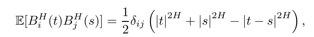
where δ is the Kronecker symbol.For each j=1,···,m,and t ∈ [0,T],letbe the σalgebra by,0≤s≤t,augmented by all the P-zero measurable events.We denote the corresponding filtration byLet W=(W1(t),···,Wm(t)),t∈ [0,T]be an F-adapted m-dimensional standard Brownian motion(sBm,for short).We say that W=(W1(t),···,Wm(t))is the underlying standard Brownian motion corresponding to BH=(BH1(t),···,BHm(t)),t∈ [0,T]if

where

We consider the following backward stochastic differential equation

where ξ is given terminal value,f and g are the given(random)generators.To solve this equation is to find a pair of adapted processes(Yt,Zt)0≤t≤T,satisfying the above equation(1.1).
Backward stochastic differential equations have a variety of applications in fields such as stochastic optimal control theory,mathematical finance,probability interpretation of solutions of quasi-linear partial differential equations and so on.The general nonlinear backward stochastic differential equations with respect to standard Brownian motions were first introduced by Pardoux and Peng[25].Peng recently gave a survey[23]on the developments in the theory of nonlinear BSDEs during the past 20 years,including the existence and uniqueness of the solutions,nonlinear Feynman-Kac formula,nonlinear expectation and many other results in BSDEs theory and their applications to dynamic pricing and hedging in an incomplete financial market.
Because the fractional Brownian motions are not semimartingales except the case H=1/2,it can be used to describe and explain some natural or society phenomenons,such as to model hydrology,climatology,signal processing,network traffic analysis,control theory, finance as well as various other fields.This makes the stochastic analysis for fractional Brownian motions challenging and fascinating.In recent years,the stochastic integral with respect to the fBm had been investigated from different perspectives by many authors[1,9,10,20,26],and so on.For the Malliavin calculus with respect to fBm and applications,thanks to the contribution of[8,14,21,22]and references there.Hu and Peng in[17]had studied the backward stochatic differential equations driven by fractional Brownian motions.They studied the general and linear BSDEs driven by fractional Brownian motions.Shortly afterwards Fei,Xia,and Zhang in[11]had analogous results as Hu and Peng in[17]to the BSDEs driven by both standard and fractional Brownian motions.In both articles,the pair of solutions of BSDEs(Yt,Zt;0≤t≤T)relied on the simple process ηt= η0+b(t)+where b and σ are determinate function in L2([0,T]).In this article,we will cancel this dependency.
Especially,in stochastic optimal control theory for controlled system,BSDEs as the adjoint equations corresponding to the state equations to describe optimal control problem are essential,for example,[2–6,13,18,19,24].Recently,Han,Hu,and Song[12]obtained a stochastic maximum principle for a stochastic control problem and their adjoint backward stochastic differential equation is linear driven by the fractional Brownian motions and its underlying standard Brownian motions.They gave the explicit form solution.Furthermore,we will show the local existence and uniqueness of solutions to the general nonlinear BSDEs driven by the fractional Brownian motions and its underlying standard Brownian motions.Diehl and Friz in[7]had studied some similar equations,which used a rough paths point view.The results of Diehl and Friz were less general than those proved in this article as g were not allowed to depend to Z.
This article is arranged as follows.In Section 2,we introduce some basic notations concerning the fractional Brownian motions,standard Brownian motions,and Mallivian calculus taken from[8,10,14,21].In Section 3,we will give some results concerning stochastic differential equations driven by both fractional and standard Brownian motions.We prove the generalization of the Itˆo formula of an Itˆo type process involving the stochastic integral with respect to both standard and fractional Brownian motions.Moreover,we obtain the product formula as the corollary.In Section 4,we prove the local existence and uniqueness of the solutions to the above BSDEs(1.1)under some reasonable assumptions.
2 Preliminaries on fBm,sBm and Malliavin Calculus
Let{ρ1,···,ρk,···}be an orthogonal basic of L2([0,T])such that ρk,k=1,2,···,are smooth functions on[0,T].Let PTrepresent the set of all polynomials of standard Brownian motion over interval[0,T].Namely,PTcontains all elements of the form
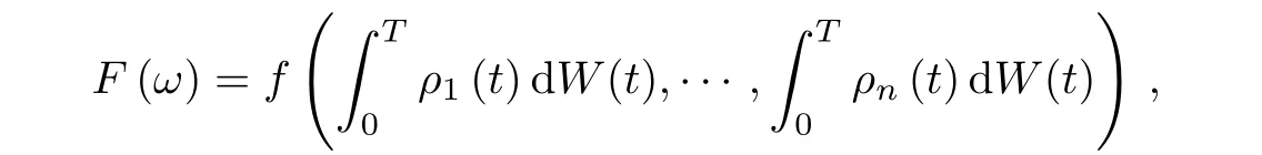
where f is a polynomial of n variables.The Malliavin derivative Dtof a polynomial functional F of standard Brownian motion is defined as

For any F∈PT,we denote the following norm

Let D1,2denote the Banach space obtained by completing PTunder the norm ‖ ·‖1,2.
Let ξ and η be two continuous functions on[0,T].Define a Hilbert scalar product

where φ :[0,T]→ R+satisfy

When ξ= η,we define the Hilbert norm by

We denote Θtas the completion of the continuous functions under this Hilbert norm.
Let{η1,···,ηk,···}be an orthogonal basic of ΘTandbe the set of all polynomials of fractional Brownian motion over interval[0,T].Namely,contains all elements of the form
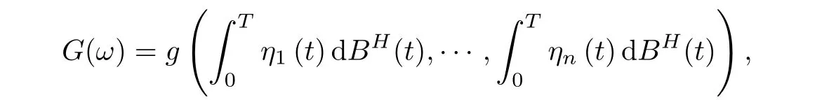
where g is a polynomial of n variables.For any G∈,the Malliavin derivativeof a polynomial functional G of fractional Brownian motion of Hurst parameter H is defined by

Introduce another Malliavin derivative


Let DH,1,2denote the Banach space obtained by completingunder the norm ‖ ·‖H,1,2.We can certainly define the higher derivatives and the space Dk,pand space DH,k,p.But we only need the space D1,2and DH,1,2in this article.


where BH(t)is a fractional Brownian motion and W(t)is the corresponding to BH(t),underlying standard Brownian motion.
Next,let us recall that the framework of stochastic integral with respect to fractional Brownian motion.The following result is well known in[10,14,15].
Proposition 2.1If Fsis a continuous stochastic process such that

then,the Itˆo-type stochastic integral can be defined under πn:0=t0< t1< ···< tn=T of the partition of the internal[0.T]:
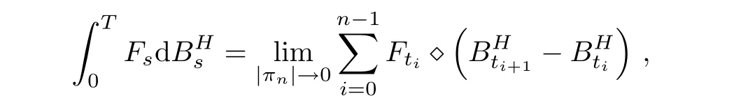
where⋄denotes the Wick product.Furthermore,we have

and

Let La(Ω;R)be the family of stochastic processes on[0,T]such that La(Ω;R)if F is R-valued,F-adapted random variable,satisfying condition(2.4).
We need the following integration by parts formula.
Proposition 2.2(see[8],Theorem 3.15)Let F∈D1,2and let(u(t),t∈[0,T])be a Itˆo integrable stochastic process such that(Fu(t),t∈[0,T])is Itintegrable.Then,

Another proposition is well known from(see[14],Theorem 10.2).
Proposition 2.3Let F∈DH,1,2and let(f(t),t∈[0,T])be(not necessarily adapted)stochastic process such that f satisfies condition 2.4.Then,

3 Itˆo Formula With Respect to Both fBm and sBm
In this section,we will give some important results concerning stochastic differential equations driven by both fractional and standard Brownian motions that will be used in the sequel.
Now,we give the generalization of the Itˆo formula of an Itˆo type process involving the stochastic integral with respect to both fractional and standard Brownian motions.
Theorem 3.1Let Gt∈(Ω;R),Ft∈ La(Ω;R)and Nt∈(Ω;R),t∈ [0,T],be real valued stochastic processes.Suppose thatAssume also thatare continuously differential with respect to(s,t)∈ [0,T]× [0,T]for almost all ω ∈ Ω.Denote
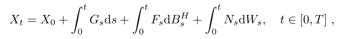
where X0is a constant.Let f be a function having the first continuous derivative with respect to t and twice continuous derivative with respect to x and suppose that these derivatives are bounded.Then,we have
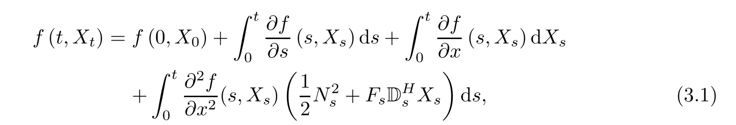
for 0≤t≤T.
ProofLet πnbe a partition defined as follows:
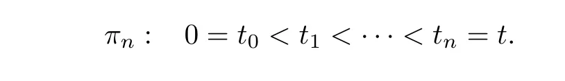
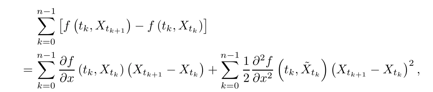
Then,we have
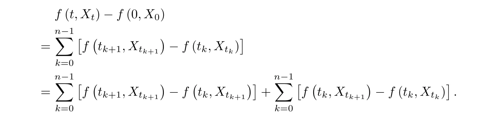
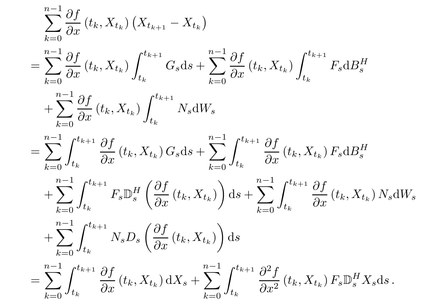
By the mean value theorem,the first sum converges to

in L2.Now,we calculate the second sum.Using Taylor′s formula and expanding each term in the sum to the second order,we obtain
Step 1Let us show that

in L2as n→+∞.We can compute the following term by formulas(2.6)and(2.7).Drut=0,if r> t,∀ ut∈(Ω;R)(see[8],Corollary 3.13).Thus,we have
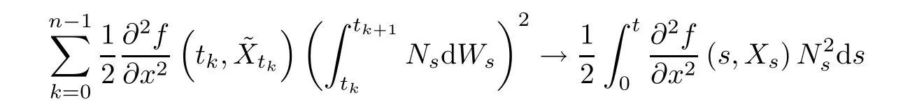
Step 2We will show that
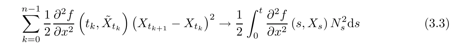
in L2as n→+∞.
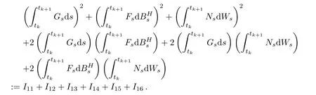
Clearly,the contribution of I14,I15,and I16to limit(3.3)is zero.We have
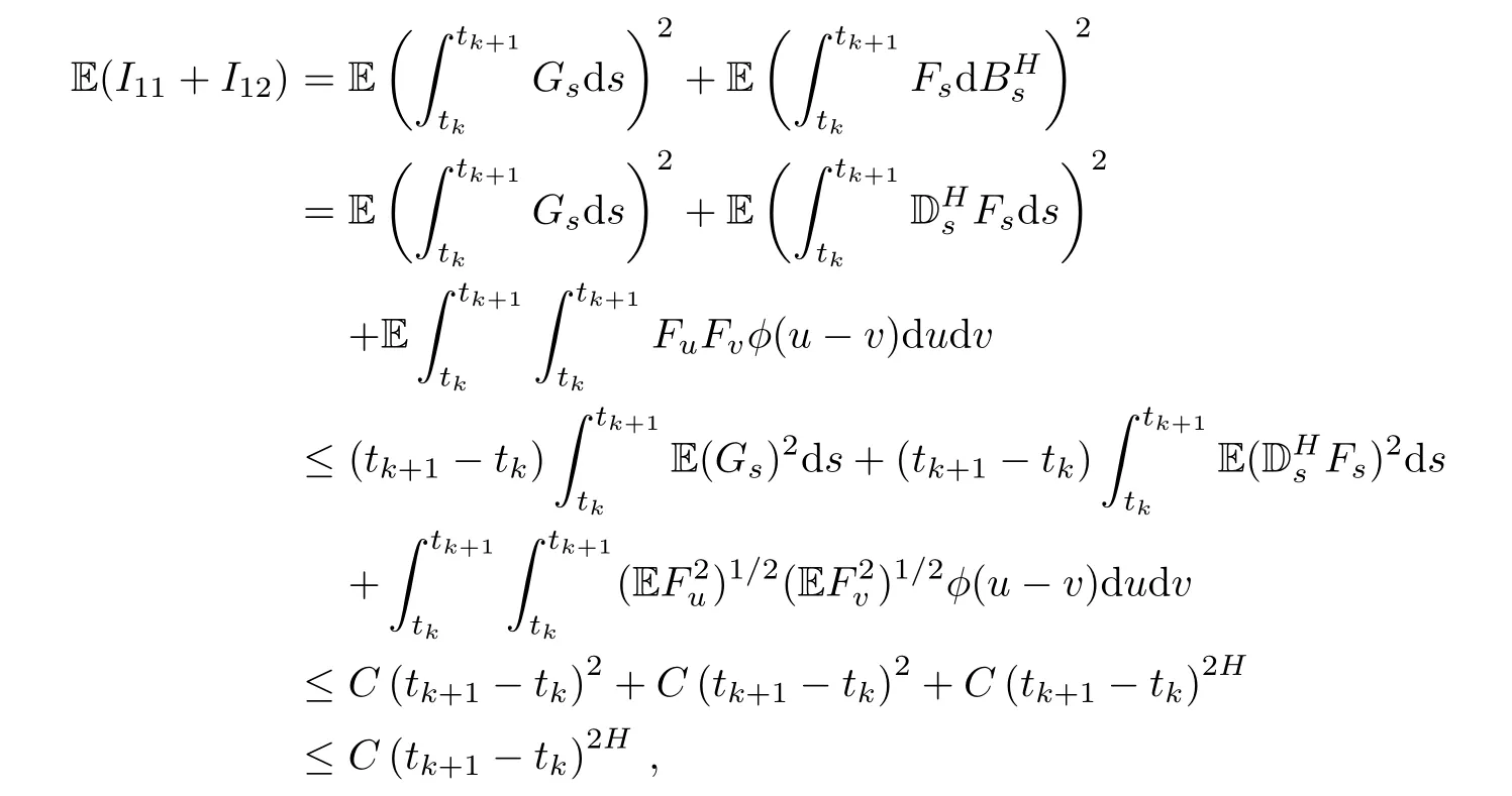
where tk+1− tk→ 0,and C is a constant independent of the partition π that may differ from line to line.
By the assumptions,we know that the second derivative of f with respect to its second variable is bounded.Thus,we have
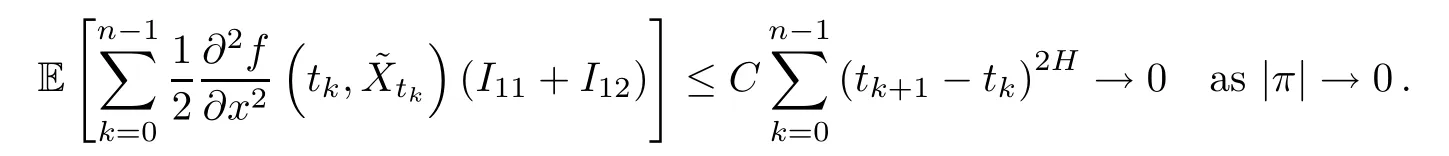
Therefore,by the isometry formula,it is easy to get
in L2as n→+∞.This completes the proof of the theorem.
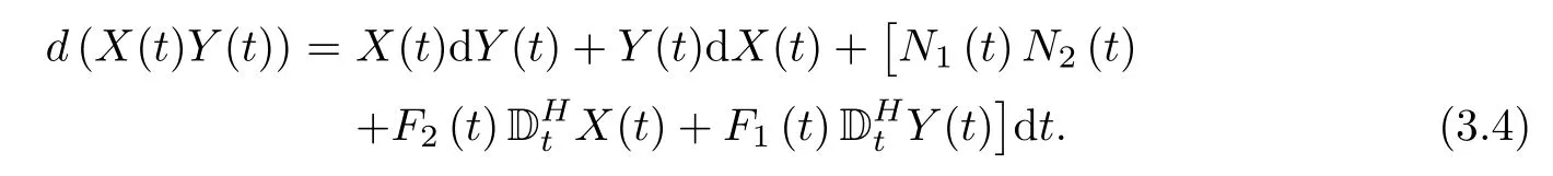
Next,we provide the product formula to stochastic differential equations with respect to both fractional Brownian motions and standard Brownian motions.It is not hard to obtain the following corollary that the function f(t,x,y)=xy under the above theorem.
Corollary 3.2Let Xtand Ytbe two processes satisfying

and

where stochastic processes Fi(t),Gi(t),Ni(t),i=1,2,satisfy the assumptions of Theorem 3.1,and X0and Y0are constants.Then,

which may be written formally as
4 Local Existence and Uniqueness of Solutions to BSDEs
In this section,we will consider the local existence and uniqueness of solutions to the following BSDEs driven by the fractional Brownian motions and the underlying standard Brownian motions.
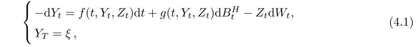
where T ∈ (0,+∞)is bounded time to be con firmed.The generator f:[0,T]×Rn×Rn×m→Rnand g:[0,T]×Rn×Rn×m→ Rn×mare given(random)functions.ξ∈(Ω;Rn)is a given terminal variable.Without lose of generality,we let n=m=1.

We have the following assumptions on the generator f and g.
Assumption(H):
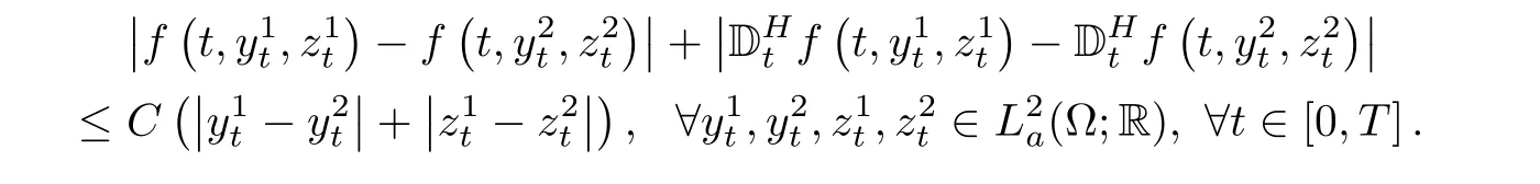
(H1)f(t,y,z)∈(Ω;R)is continuously differentiable,and mean square bounded.Its Malliavin derivatives exists,satisfyingMoreover,the Lipschitz conditions hold for f andThat is,
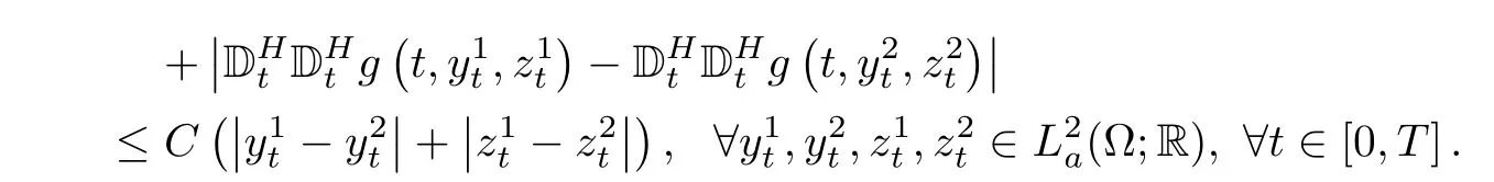
(H2)g(t,y,z)∈ La(Ω;R)is twice continuously differentiable with respect to y and z,and itsfirst and second-order Malliavin derivatives exist,all of which are mean square bounded.Moreover,there exists a constant C>0 such that the following inequality hold:

Definition 4.1A solution to BSDE(4.1)is a pair of stochastic processes(Yt,Zt)0≤t≤T∈and the pair of processes satisfies

Theorem 4.2Suppose that(H1)and(H2)hold.Then,there exists uniquely a pair of solutionto BSDE(4.1)with any terminal value
To prove Theorem 4.2,we consider firstly the simple case of f(t,yt,zt)=f(t)and g(t,yt,zt)=g(t).That is,BSDE(4.1)has the following form

Lemma 4.3Assume that ft∈and gt∈ La(Ω;R).Then,there exists uniquely a pair of solutionof BSDE(4.2).
ProofThe proof of the uniqueness is obvious.We omit it.For the existence of the solution,we show the following statement.Let
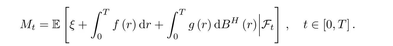
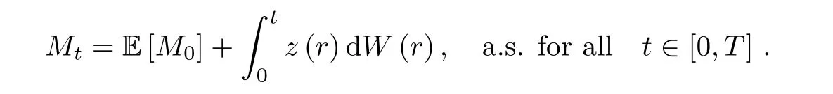
It is easy to see that Mtis a Ft−martingale.With the martingale representative theorem,there exists a unique stochastic process zt∈for all 0≤ t≤ T.Moreover,
Next,we define ytas follows:
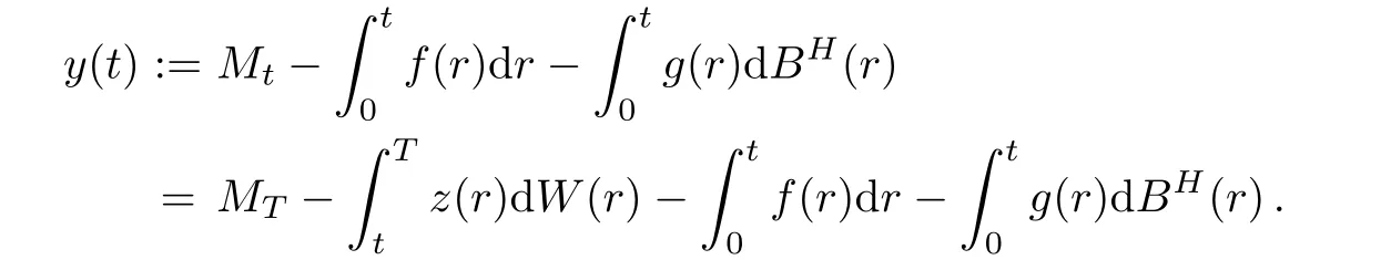
It is easy to see that y(t)∈Furthermore,is the solution of BSDE(4.2).
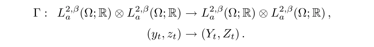
For each(yt,zt)→ (Yt,Zt),we know that BSDE(4.1)has a pair of solutionby Lemma 4.3.Let Γ be the map defined as follows,
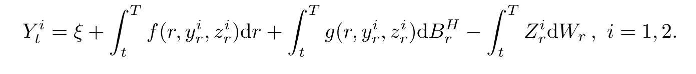
To complete the proof of Theorem 4.2,what we need is to prove that the map Γ is contractive.Suppose thatandare solutions of BSDE(4.1),corresponding to(yt,zt)=respectively.Then,we have
Let
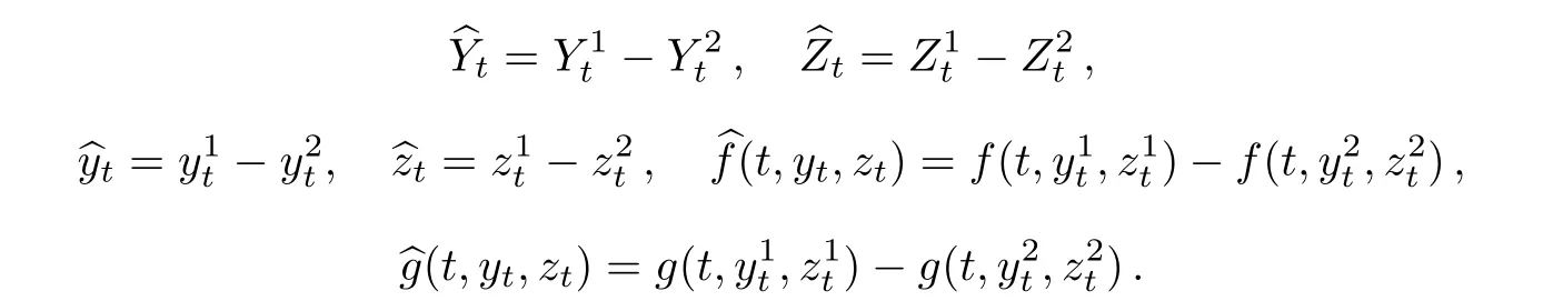
We have

Now,the proof will be decomposed in several steps.
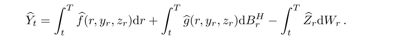
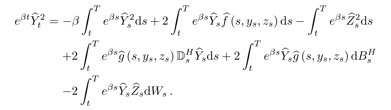
Step 1The integral form can be written by
It is well-known that DrXt=0,if r> t,∀Xt∈We have the following equations by(2.6),(2.7),and(2.3).

The Malliavin derivative can be expressed with(2.2)and(2.3)by
Thus,
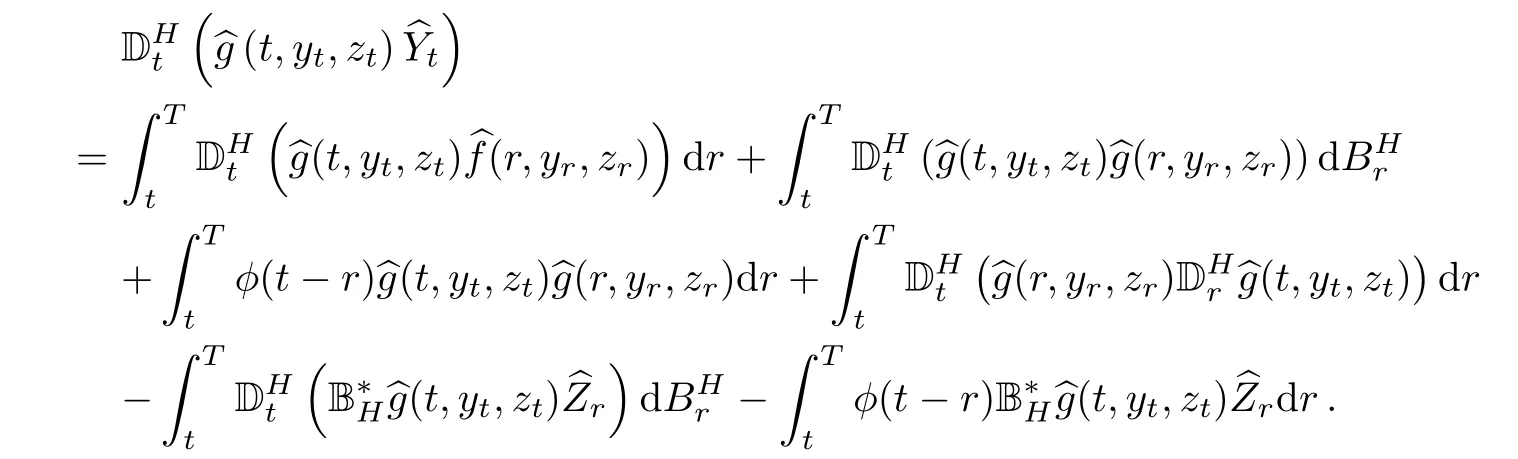
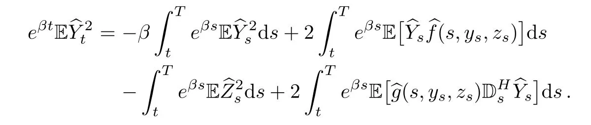
Step 2By formula(3.4),we have

Again using the product formula,we have
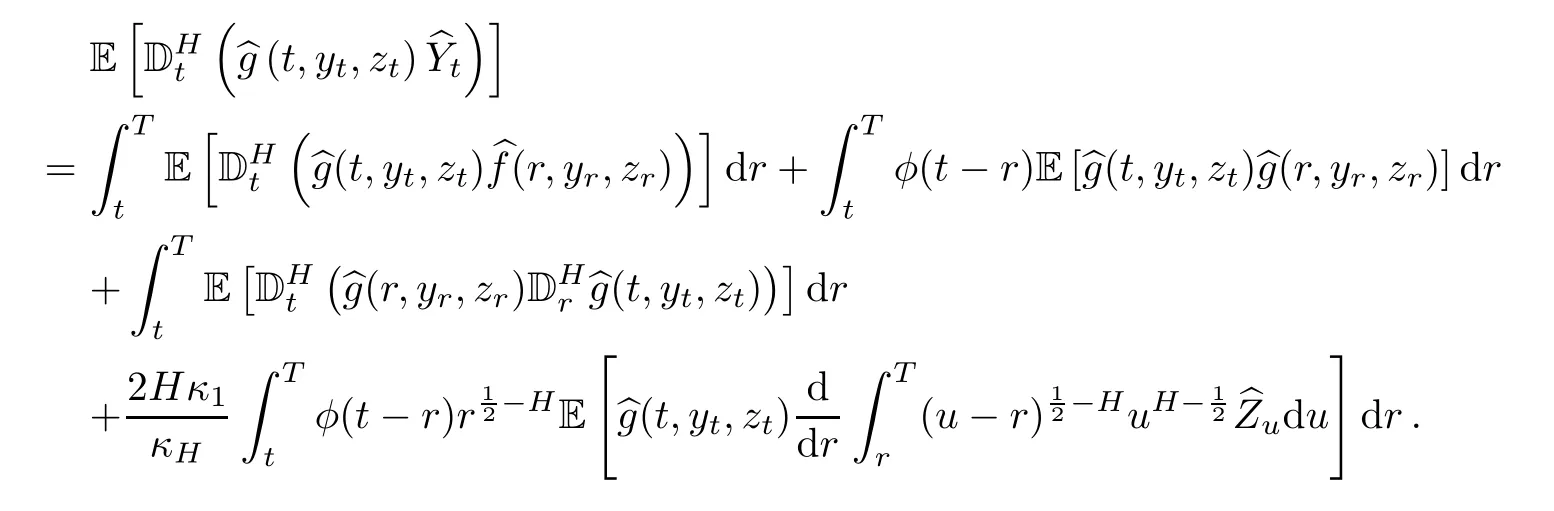
Taking expectation,we obtain
So,we have
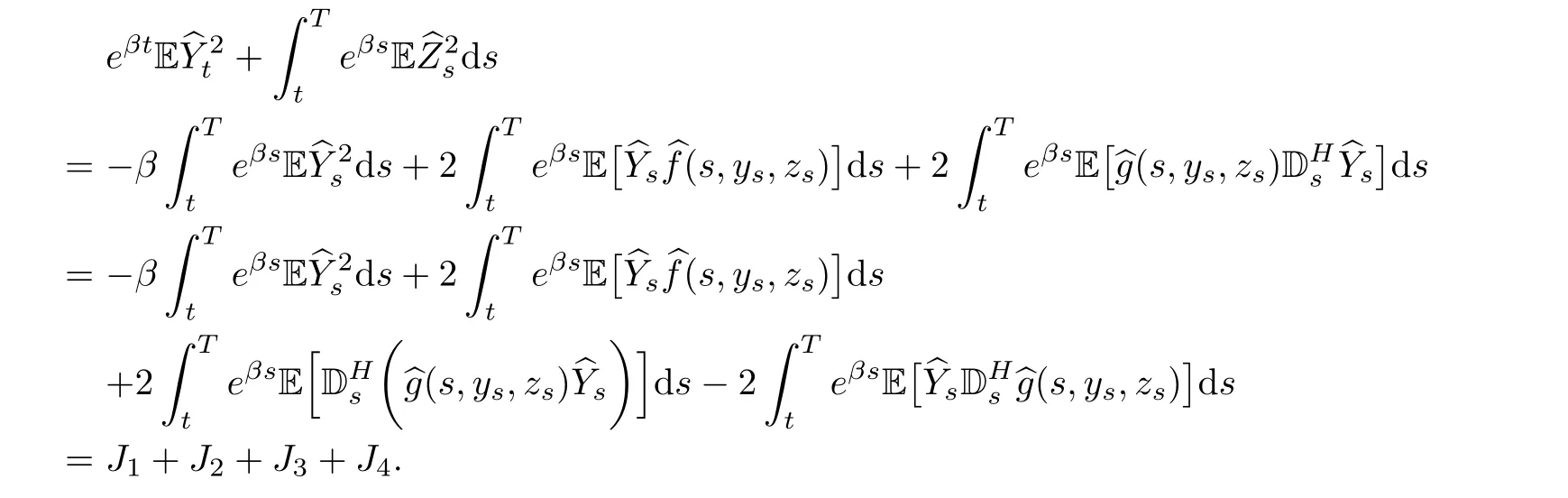
Step 3Firstly,we calculate J1+J2+J4.

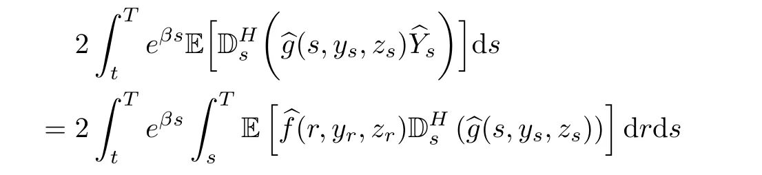
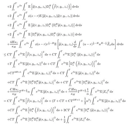
Now,we can group
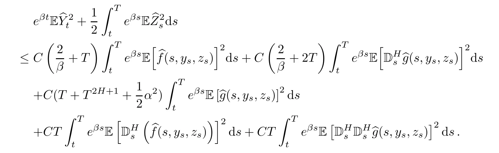
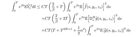
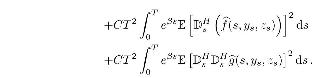
We also have
Summarizing with Assumption(H),we obtain

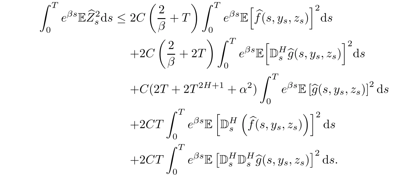
where

So,we only need to choose T small enough and β big enough,satisfying that CQ < 1.Then,we complete the proof of Theorem 4.2 by using of contractive mapping principle.
[1]Alòs E,Nualart D.Stochastic integration with respect to the fractional brownian motion.Stoch Stoch Rep,2003,75(3):129–152
[2]Bender C.Explicit solutions of a class of linear fractional BSDEs.Systems Control Lett,2005,54(7):671–680
[3]Bensoussan A.Lectures on Stochastic Control.Lecture Notes in Math.Berlin-New York:Springer,1982
[4]Biagini F,Hu Y,Øksendal B,Sulem A.A stochastic maximum principle for processes driven by fractional brownian motion.Stochastic Process Appl,2002,100:233–253
[5]Bismut J M.Conjugate convex functions in optimal stochastic control.J Math Anal Appl,1973,44:384–404
[6]Bismut J M.An introductory approach to duality in optimal stochastic control.SIAM Rev,1978,20(1):62–78
[7]Diehl J,Friz P.Backward stochastic differential equations with rough drivers.Ann Probab,2012,40(4):1715–1758
[8]Di Nunno G, Øksendal B,Proske F.Malliavin calculus for Lévy processes with applications to finance.Berlin:Springer-Verlag,2009
[9]Dai W,Heyde C C.Itˆo formula with respect to fractional brownian motion and its application.J Appl Math Stochastic Anal,1996,9(4):439–448
[10]Duncan T,Hu Y,Pasik-Duncan B.Stochasticcalculus for fractional brownian motion I.theory.SIAM J Control Optim,2000,38(2):582–612
[11]Fei W,Xia D,Zhang S.Solutions to BSDES driven by both standard and fractional brownian motions.Acta Math Appl Sin Engl Ser,2013,29(2):329–354
[12]Han Y,Hu Y,Song J.Maximum principle for general controlled systems driven by fractional brownian motions.Appl Math Optim,2013,67(2):279–322
[13]Haussmann U G.General necessary conditions for optimal control of stochastic system.Math Programm Stud,1976,6:34–48
[14]Hu Y.Integral transformations and anticipative calculus for fractional brownian motions.Mem Amer Math Soc,2005,175(825)
[15]Hu Y,Øksendal B.Fractional white noise calculus and applications to finance.In fin Dimens Anal Quantum Probab Relat Top,2003,6(1):1–32
[16]Hu Y,Øksendal B.Partial information linear quadratic control for jump diffusions.SIAM J Control Optim,2008,47(4):1744–1761
[17]Hu Y.Peng S.Backward stochastic differential equation driven by fractional brownian motion.SIAM J Control Optim,2009,48(3):1675–1700
[18]Hu Y,Zhou X.Stochastic control for linear systems driven by fractional noises.SIAM J Control Optim,2005,43(6):2245–2277
[19]Kushner H J.Necessary conditions for continuous parameter stochastic optimization problems.SIAM J Control,1972,10:550–565
[20]Lin S.Stochastic analysis of fractional Brownian motions.Stochastics Stochastics Rep,1995,55(1):121–140
[21]Nualart D.The Malliavin calculus and related topics.Berlin:Springer,2006
[22]Nualart D,Rascanu S.Differential equations driven by fractional brownian motion.Collect Math,2002,53(1):55–81
[23]Peng S.Backward stochastic differential equation nonlinear expectation and their applications//Proceedings of the International Congress of Mathematicians Hindustan Book Agency.India:New Delhi,2010:393–432
[24]Peng S.A general stochastic maximum principle for optimal control problems.SIAM J Control Optim,1990,28(4):966–979
[25]Pardoux E,Peng S.Adapted solution of a backward stochastic differential equation.Systems Control Lett,1990,14(1):55–61
[26]Wu L,Ding Y.Wavelet-based estimator for the Hurst parameters of fractional Brownian sheet.Acta Mathematica Scientia,2017,37B(1):205–222
 Acta Mathematica Scientia(English Series)2018年2期
- Acta Mathematica Scientia(English Series)的其它文章
- ON A FIXED POINT THEOREM IN 2-BANACH SPACES AND SOME OF ITS APPLICATIONS∗
- MULTIPLICITY AND CONCENTRATION BEHAVIOUR OF POSITIVE SOLUTIONS FOR SCHRÖDINGER-KIRCHHOFF TYPE EQUATIONS INVOLVING THE p-LAPLACIAN IN RN∗
- MULTIPLICITY OF SOLUTIONS OF WEIGHTED(p,q)-LAPLACIAN WITH SMALL SOURCE∗
- QUALITATIVE ANALYSIS OF A STOCHASTIC RATIO-DEPENDENT HOLLING-TANNER SYSTEM∗
- SHARP BOUNDS FOR HARDY OPERATORS ON PRODUCT SPACES∗
- CONTINUOUS FINITE ELEMENT METHODS FOR REISSNER-MINDLIN PLATE PROBLEM∗