
Master equation and runaway speed of the Francis turbine *
2018-05-14 01:42ZhZhang
水动力学研究与进展 B辑 2018年2期
Zh. Zhang
Free Researcher, Zurich, Switzerland
Introduction
The hydraulic characteristics of a Francis turbine are generally represented by the discharge, the power output and the efficiency as a function of the hydraulic head, the angle of the guide-vanes and the rotational speed of the turbine. Because such hydraulic characteristics are closely related to the flow losses of diverse types, especially at partial loads, they could for a long time not be computed with sufficient accuracy. At best, one only knows about some of the general losses in Francis turbines which are simply operated at the best efficiency point (BEP)[1]. For partial load operation of Francis turbines, there has practically not been any reliable analytical and computational method which can be used to estimate the hydraulic performance of the turbine system. For the purposes of such estimations, therefore, experimental measurements on model turbines are virtually the only procedures. They are, however, always associated with high costs and are time-consuming. This circumstance strongly restricts the closer determination of all related flow dynamic behaviours of Francis turbines while getting started or stopped, for instance.It will also affect the accurate computations of the hydraulic transients which are related to the flow regulations by changing the guide-vane angle and/or the rotational speed.
It seems, therefore, quite indispensable to work out a reliable computational method to reveal the complex characteristics of Francis turbines. For this purpose, all types of flow losses that are related to both the changeable discharge and the changeable rotational speed need to be quantified. The dominant hydraulic losses in Francis turbines at operation points outside the design point are shock losses at the impeller inlet due to the abrupt change in the flow direction and exit flow losses. The latter are associated with the circumferential velocity component of the flow at the impeller exit and in the draft tube. In addition, the mechanical loss, which is related to the rotational speed, takes part in the efficiency loss.Basically, the shock loss at the impeller inlet can be satisfactorily determined by initially using the conservation law of momentum (Section 1.6.2). Determination of the exit flow losses, however, requires detailed knowledge on both the meridian and the tangential velocity distributions at the impeller exit,i.e., in the draft tube. Lack of the computational procedure to the flow distribution at the impeller exit has so far limited the computational estimations of the exit losses and of the hydraulic characteristics of the Francis turbine.
While the hydraulic performances of Francis turbines have been determined mainly through measurements and model tests, they are increasingly and commonly also simulated by numerical methods based on computational fluid dynamics (CFD), as can be widely found nowadays. It should be mentioned that all numerical investigations are case studies and are hardly able to reveal any significant concepts in turbine flows. Using a statistical procedure regarding measurement data at a set of pump-turbines of different specific speeds, Zeng et al.[2,3]revealed reasonable relations between the turbine characteristics and the turbine specific speed. This empirical relation,however, does not apply to Francis turbines because of different design principles and criteria.
A first breakthrough in the analytical method for turbine characteristics has been achieved by Zhang and Titzschkau[4]. The crucial point involved in the new method is the accurate computation of the exit losses at the impeller exit based on the use of the so-called streamline similarity method (SSM), which was initially and separately developed for the flow distribution at the impeller inlet of the centrifugal pump. The computational results have almost satisfactorily agreed with measurements, also thanks to the accurate computations of the shock loss at the impeller inlet. For the details about the SSMand its excellent universal applicability, the readers are kindly referred to the latest article[5]. At that time (2012) in Ref. [4], the method was only mentioned in the references as a private communication.
A special phenomenon with the operational instability is the so-called S-shape instability, when the discharge is close to zero, as for the starting process and the case of reaching the runaway speed.Despite of lots of investigations, for instance[6-8], the mechanism of such an operational instability could still not satisfactorily be revealed. Almost all research activities have again only been restricted to case studies, i.e., to the characterisations of the related flow instabilities, either numerically or experimentally[9-11].The statistical description of the flow instabilities can again be found in Refs. [2, 3] based on measurements at a set of pump-turbines.
The SSM[5]shows its great advantages and its potentials of applicability in the computations of all flow quantities and hydraulic performances of Francis turbines. This also includes accurate computations of the runaway speed for load rejection at the generator.As stated in Ref. [5], there is a good prospect of using the streamline similarity method to standardize the geometrical design and to perform the advanced hydraulic computations both for pumps and turbines.For this reason, the entire mechanical background should be revealed, in order to represent them in simple and standardized form. Thus, the present paper aims to provide a complete document by improving and extending the main computations in Ref. [4]. This serves as the kick-off for a further series of investigations, including the flow instability in the near region of the S-shaped characteristic.
Physically, the flows in the Francis turbine are governed by the energy and the angular momentum(Euler) laws. For applying the energy law, obviously,one needs to quantify all available losses which exist in the turbine system. The basic computational scheme for deriving the master equation, thus, is as follows:
(1) Computing the shock loss at the impeller inlet.
(2) Computing the swirling loss at the impeller exit.
(3) Computing the friction loss as a function of the discharge.
(4) Creating the energy equation with respect to all existing losses.
(5) Computing the Euler equation with averaged exit flow distribution
(6) Then combining the energy and Euler equations to obtain the Master Equation of the Francis turbine.
(7) Resolving the discharge from the master equation.
(8) Computing the hydraulic characteristics of a given Francis turbine.
(9) Finally, computing the runaway speed based on the hydraulic characteristics.
All these steps form the main content of the present paper.
Because the complete characteristics of a Francis turbine also include the variation of the rotational speed, the definition of the nominal operation point of the Francis turbine needs to be extended, as this will firstly be considered in the next section.
1. Flow mechanical analysis
1.1 Extension of the nominal operation condition
Each Francis turbine is designed for a given nominal, i.e., rated operating point which is specified by the nominal head, the nominal discharge and the nominal rotational speed. The last is usually fixed to the synchronous speed of the generator and, thus,determined by the line frequency and the pole pair number of the generator. The designed operation condition ensures the maximum hydraulic efficiency and is realised by the shockless flow at the impeller inlet (β1=β1bin Fig.1) and the non-swirling flow at the exit (α2= π/2). Deviations from the designed operating point are encountered, for instance, by the season-dependent height of water in the lake or by changing the guide-vane angle to regulate the discharge. The former leads to the change in the effective head of the turbine. The latter aims to regulate the turbine load. All these deviations in the turbine operation happen at the constant, i.e., synchronised rotational speed.
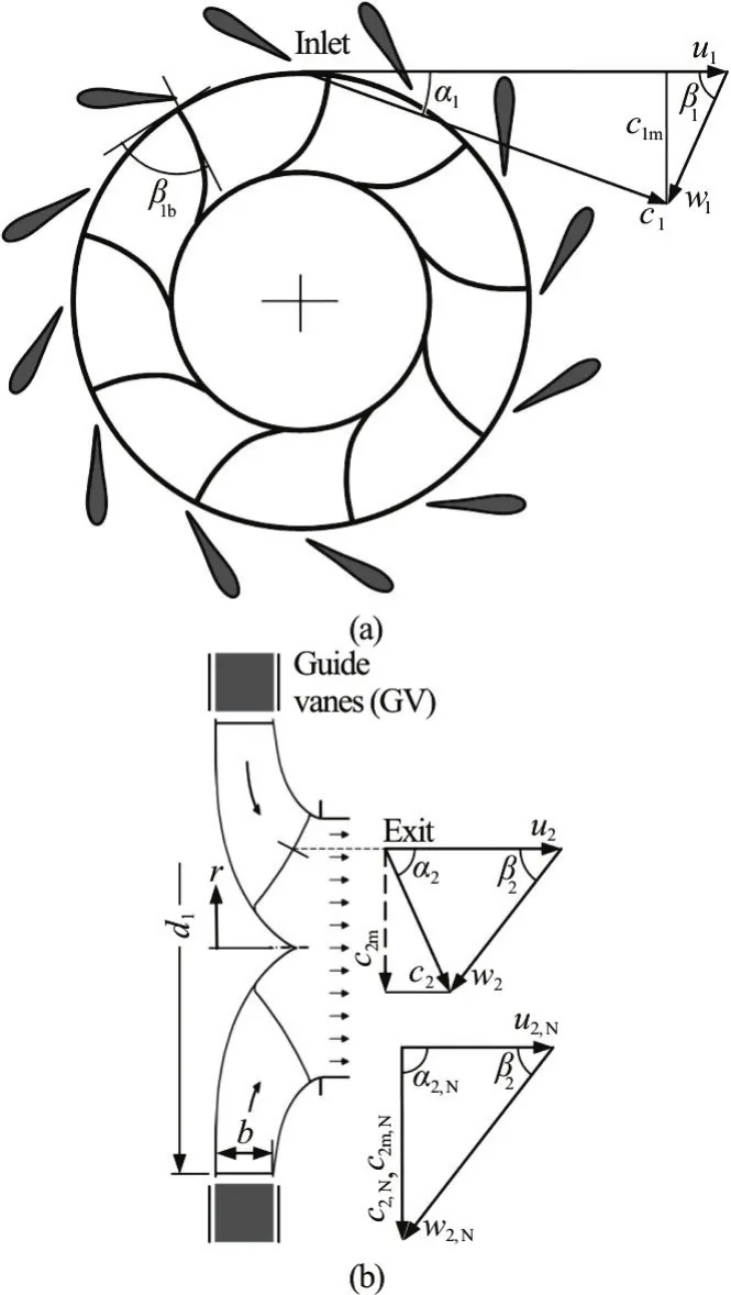
Fig.1 Velocity triangles at the impeller inlet and exit of a Francis turbine (α1 as the given flow angle)
The complete hydraulic characteristics of a Francis turbine also account for the case of changeable rotational speed. This relation is obvious,because the hydraulic transients, either during the start-up of the turbine or in the case of the load rejection leading to the runaway speed, are all highly dynamic and significant. They, therefore, require accurate descriptions. For this purpose, as in the present paper, the definition of the nominal operation condition of the Francis turbine has to be extended to include both the changeable head and the rotational speed. This simply means that to each given head a new fictitious nominal operating point regarding the speed and the discharge should exit. On the other hand,turbine operations with variable speed (Varspeed),indeed, have also been well established in practical applications[12-14]. For this reason and to extend the nominal operation conditions, the following dimensionless characteristic numbers, respectively, for rotational speed, discharge, and hydraulic torque are defined:
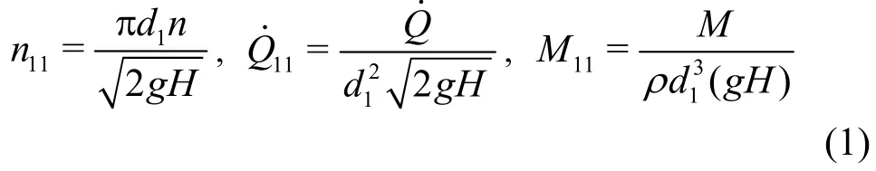
In these definitions, ρ is the density of water. Use of the impeller diameterd1as reference length, instead of the draft tube diameterd2[4], will significantly contribute to the simplification of all computational results, including those in a series of investigations regarding the runaway speed of Francis turbines. The author would also like to justify the use of dimensionless characteristic numbers. In many other applications, the respective characteristic numbers have been defined without accounting for the gravity constant. For applications with much more mathematical complexity, however, the dimensionless expressions will desirably lead to much simpler expression of the computational results, as demonstrated in the current paper.
In describing the characteristics of the Francis turbine, one also uses the discharge and the head coefficients which are, respectively, defined as:

withA1andu1, respectively, as the flow area at the impeller inlet and the peripheral speed of the impeller(Fig.1). The definition of the head coefficient is equivalent to that of the unit rotational speed because of
Departing on the definitions of Eq. (1), corresponding values under nominal operation conditions are denoted byn11,N,1,NandM11,N. This simply means that to each given hydraulic head there exists a new nominal operating point, which is completely analogous to the designed (rated) operating point with the designed head. The extended nominal operating condition is thus implemented by accounting for the variable head.
Correspondingly, the nominal discharge coefficient is given as
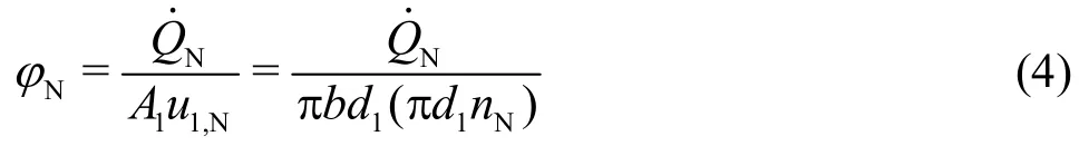
From Eqs. (1) and (4), one obtains

Since the discharge coefficient φN, due toN=c1m,NA1, can also be represented as φN=c1m,N/u1,N, it follows from Fig.1 directly
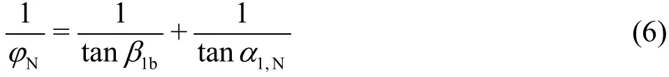
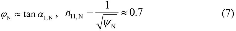
The nominal discharge coefficientNφ is a design parameter of a Francis turbine and represents the combination of β1band α1,Nor, alternatively, ofn11,Nandaccording to Eq. (5). Its application in the frame of the present paper contributes to the simplification of computational results. One thing worth mentioning is that the nominal head coefficient Nψ as another design parameter has also been very often used in Francis turbines. In reality, it is related to theunit speedby. For a special design of the Francis turbine with β1b≈ π/2, there is ψN≈2 when assuming ηhyd,N≈ 100%. Thus, it straightforwardly follows that
Referring to Eqs. (1) and (5), the nominal unit dischargeis determined by the nominal dischargeand the actually available hydraulic headH.The same also applies ton11,NandM11,N. One confirms from Eq. (5), for instance, that the new nominal dischargeis tightly connected with the new nominal rotational speednN. From Eq. (6), one further confirms that the nominal flow angle α1,Nis a fixed geometrical parameter and thus independent of the head. Usually, the flow angle downstream of the guide vanes differs from the guide-vanes setting angle.In the frame of the current paper, as in common practice, the flow angle α1is occasionally also called the setting angle of the guide vanes. In addition,the term “nominal”, instead of “rated” or “designed”,is used to generally represent the best efficiency point(BEP) of the Francis turbine, with variable rotational speed.
1.2 Impeller design and flow distribution at the impeller exit
The basic parameters for the design of a Francis turbine are the nominal head, the nominal discharge and the nominal rotational speed. By applying these three parameters, the specific speed of the Francis turbine is defined as follows

It is a fixed parameter which basically determines the geometrical form of the impeller of the Francis turbine.As can be easily confirmed, the specific speed remains unchanged when both the nominal discharge and the nominal rotational speed change with the head by satisfying the conditions=constant andn11,N=constant.
In the practical design of the Francis turbine, the head coefficient ψNhas been arranged as a function of the specific speednq. With respect to ψN=andn11-definition according to Eq. (1), the diameter of the impellerd1can be determined. For other parameters, corresponding determining equations and diagrams can be found in the literature. This,however, is not within the scope of this paper. The case to be currently considered is the geometrical design of the impeller blades at the impeller exit. This is simply because such a geometrical design crucially determines the exit flow distribution and further the characteristics of the Francis turbine.
The exit profile of the impeller blades is designed for the nominal operation of the Francis turbine. It enables the exit flow out of the impeller to be free of circulations and to consist only of the meridian velocity component. The velocity distribution in the meridian plane, because of streamline curvatures, is non-uniform and depends on the in-plane profiles on both the shroud and hub sides of the impeller (Fig.1).It should be, however, of the type of the potential flow distribution, because the expected downstream flow in the draft tube is uniform and thus of potential flow character. Such a flow distribution at the impeller exit is, thus, comparable to the inlet flow at a centrifugal pump. Corresponding accurate analyses, as given in Ref. [5] for the pump flow, can thus be applied. One obtains the velocity distribution along the trailing edge of the impeller blade as
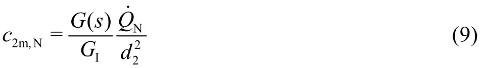
In this equation,G(s) represents a geometrical variable along the trailing edge of the impeller blade and is computed by
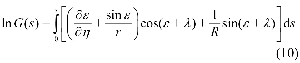
in whichRis the radius of curvature of the streamlines.
The geometrical constantGIbalances the mass flow and is called the first structural constant, given as
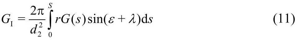
For a given meridian profile of the impeller at the impeller exit, bothG(s) andGIcan be numerically computed, for instance, simply by means of the use of MS Excel. Corresponding computational algorithms can be found in Ref. [5].
Based on the velocity distribution in the meridian plane, i.e.,c2m,Naccording to Eq. (9), the radial profile of the impeller blade along the blade trailing edge can be computed. The representative parameter is the trailing angle of the blade2β. According to Fig.1(b) for the nominal flow condition (α2=π/2), this is computed as
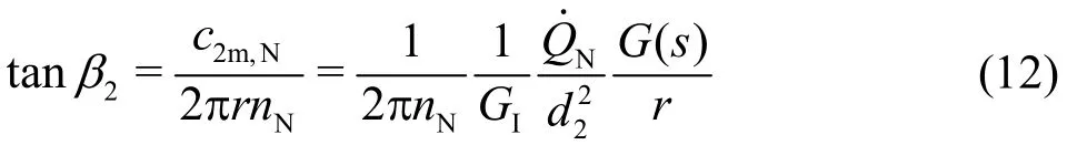
With respect to Eqs. (1) and (5), this formula can also be expressed in terms of the characteristic numbersandn11,Nas well as of the discharge coefficient φN. It represents the design rule for the radial profile of the impeller blade at the impeller exit. As can be confirmed, such a profile is independent of the flow at the impeller inlet. The geometrical variableG(s) along the trailing edge of the impeller blade can also be written asG(r), so that the radial distribution of β2(r) is obtained.
At other operation points deviating from the nominal condition, the exit flow out of the impeller possesses a circumferential velocity component. The distribution of the meridian velocity component in the meridian plane, however, can still be considered to be of the potential flow character. It is, thus, analogous to that under the nominal condition and can be written as
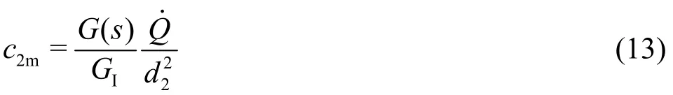
Accurately expressed, the similarity of the velocity distribution to the case of the nominal flow is only a hypothesis. At deep partial loads, for instance, the flow separation at the impeller inlet will more or less affect the meridian velocity distribution at the impeller exit. On the other hand, as will be shown below, Eq.(13) will be used, as a weighting factor, only to weight the circumferential velocity component and the related kinetic energy at the impeller exit. For this reason, the inaccuracy of the assumed velocity distribution in the above equation will only insignificantly influence the computations of integration. In reality, the velocity distribution given in the above equation could indeed be verified by experiments, even only indirectly. As a type of potential flow, the velocity distribution given in Eq. (13) should become uniform while entering the draft tube. Such a uniform velocity distribution in the draft tube, except in the near region of the tube axis,has already been well demonstrated in Ref. [15].
The law of the velocity distribution according to Eq. (13) has its computational background that it significantly contributes to further simplifications of all computational results. Anyhow, the computational results and the comparison with measurements will finally verify the hypothesis made in Eq. (13).
Furthermore, the relative flow at the impeller exit can still be considered to follow the blade profile. The absolute flow velocity, then, comprises the circumferential component (in Fig.1(b),2α≠π/2). Theoretically this is given by

This velocity distribution can in reality not be fully true. While the flow at the impeller inlet is considered to be a potential flow and the viscous effects on the flow distribution within the impeller are negligible,the flow at the impeller exit has to be of the same potential character. This means that the circumferential velocity componentc2ushould be inversely proportional to the radial coordinate. Such a flow trend will more or less distort the flow distribution given in the above equation. For this reason, the above equation is modified to
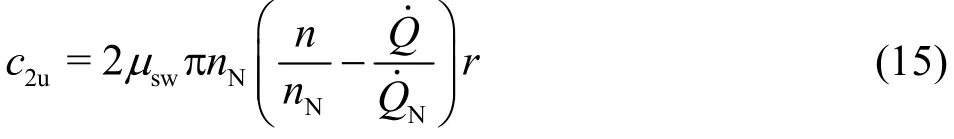
The factor μswcorrects the distribution of the velocity component which is related to the swirling flow. It is smaller than unity and should be determined in connection with the averaged values likeand. In Section 4, showing the application example, the factor μswhas been individually found to be μsw≈ 0.85.
Further, because of Eqs. (2) and (4), one obtains

It is linearly proportional to the radial coordinate and represents a flow rotation like a solid piece.
Equation (16) indicates also physically that the dimensionless tangential velocity component at the impeller exit is only a function of the discharge coefficient and thus independent of the head coefficient.This statement has been exactly verified by measurements[15]. There, one also made the same statement and experimental verification for the meridian velocity component which is given by Eq. (13). It can, thus, be concluded that the velocity distribution at the impeller exit only depends on the discharge coefficient.
1.3 Euler equation and specific work
The Euler equation basically represents the angular momentum law and specifies, in its given form, the energy exchange between the fluid flow and the impeller of the Francis turbine. The specific work conducted by the flow in the Francis turbine is accordingly given by

The hydraulic efficiency of the Francis turbine is denoted by ηhyd. If the head is considered to be that between the turbine inlet and the lower reservoir, then the hydraulic efficiency also accounts for the loss in the draft tube. This is the common case, because the draft tube always belongs to the unit of the Francis turbine. Furthermore,c1uis the circumferential component of the uniform flow velocity at the impeller inlet. Forc2usee Eqs. (15) and (16).
The averaged term, which is related to the exit flow out of the impeller, must be computed by integrating the non-uniform flow distribution along the trailing edge of the impeller blades froms=0 tos=S(Fig.2). This is given by

The meridian velocity is used here for weighting purposes. According to Eq. (13) forc2mand Eq. (15)forc2uas well as withu2=2πrn, one obtains
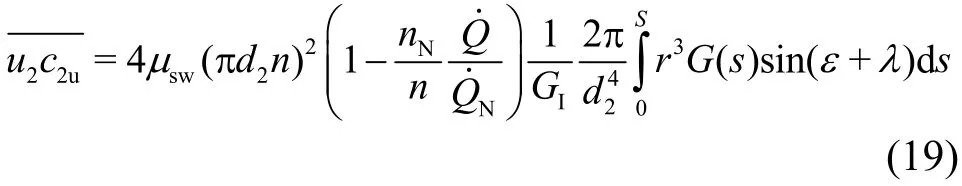
Obviously, the integration term again represents a geometrical quantity. It is denoted byGΙI, in dimensionless form as
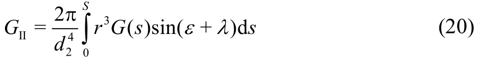
which is called the second structural constant[5]and balances the mean value of the specific energy.

Fig.2 Dimensioning of the impeller and exit flow along the trailing edges of the impeller blades
Finally, one obtains

The considered discharge above is obviously related to the flow through the impeller. It differs from the discharge through the turbine by the leakage flow through the side-wall of the impeller. For not too small discharge, this difference can be neglected.However, under the condition beyond the runaway speed or at closed guide vanes, backward flow through the impeller might occur and the volumetric flow rate is comparable to the rate of the leakage flow.Such conditions represent the well-known S-shape instability of the discharge characteristics and have been widely investigated. For the sake of simplicity in deriving both the master equation of the Francis turbine and the discharge characteristics, the leakage flow will be neglected. This means that the computations in the upper range of the rotational speed,i.e., beyond the runaway speed would suffer from some errors.
1.4 Hydraulic efficiency and the structural constant of the impeller
In usingu1=πd1nandc1u=c1m/tanα1, which are related to the velocity triangle at the impeller inlet,and with respect to Eq. (21), the hydraulic efficiency of the Francis turbine is computed from Eq. (17) as
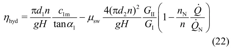
With respect to the characteristic numbers defined in Eq. (1) and because of=A1c1m=πd1bc1m, it then follows from the above equation

in which the structural constantGof the impeller is defined as
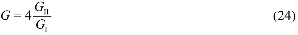
It represents the significant geometrical design parameter, which also directly determines the runaway speed of the Francis turbine, see Section 3 below.
Under nominal flow conditions, the exit flow out of the impeller does not possess any circumferential velocity component, so that the second term on the r.h.s. of Eq. (23) disappears. With respect to Eqs. (5)and (6) one obtains
1.5 Rate of angular momentum and torque
For the purpose of conducting further analyses in subsequent investigations, the angular momentum embedded in the flow at the impeller exit should be given here. While the rate of the angular momentum at the impeller inlet is simply given by=, the corresponding value at the impeller exit must be computed from the integration because of the non-uniform velocity distribution there; this is given by
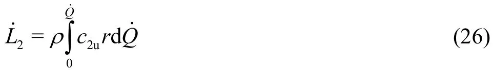
Following the same computational procedure that led to Eq. (21), one obtains

The hydraulic torque is determined by the difference between the two angular momentum flow rates (and). Withc1u=c1m/tanα1, the torqueMhydfollows as
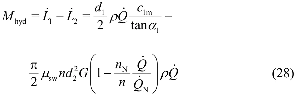
With respect to Eq. (1), this equation is further rearranged to the expression

This equation has the property that forM11,hyd=0,there are two values of. The first is found atwhich is related to the runaway speed,and the second is=0, which is found beyond the runaway speed and represents the transition of the turbine mode into the pump mode. The latter withM11,hyd=0, however, has never been observed in practice, even after subtracting the mechanical losses.The reason mainly lies in the leakage flow which circulates between the impeller channels and the impeller’s side-wall gap. In fact, such a flow circulation occurs, as long as the discharge of the turbine is smaller than the leakage flow. The mechanism of the related reverse flow within the impeller totally differs from that leading to Eq. (29). Thus, a special flow model has to be built in the future.
On the other hand, the representative exit of the impeller actually lies at the inlet of the draft tube where the flow contraction is finished and the radial velocity component vanishes. The flow from the trailing edge of the impeller blades to the inlet of the draft tube can be considered to be free of any losses.Furthermore, the rate of the angular momentum must remain constant, which implies the change of the radial distribution of the circumferential velocity componentc2u. This change can be computed by assuming its proportionality and the uniform distribution of the axial flow in the draft tube. Thus, one first obtains
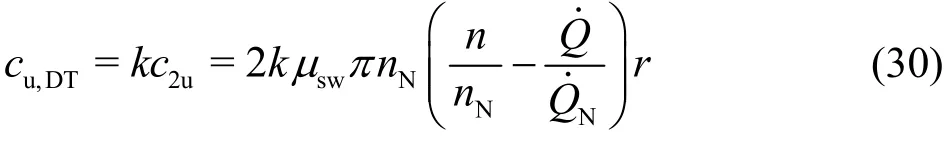
The proportional constantkcan be determined from the unchanging rate of the angular momentum. From Eq. (30) and under the assumption of uniform distribution of the axial flow (cm,DT), the angular momentum at the inlet of the draft tube is computed,with, as
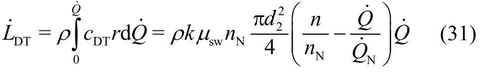
From, it follows

Thus, one obtains
This distribution will be used to compute the related kinetic energy, which has to be considered to be the loss, see Section 1.6.3 below.
Equation (32) undoubtedly demonstrates the significance of using the structural constantG.
1.6 Examination of existing flow losses
The hydraulic efficiency of a Francis turbine can be computed if all hydraulic losses are known.Basically, the possible hydraulic losses can be catego rised into the flow-dependent friction-dominant losses and the losses which only occur when the turbine is operated at the points out of the nominal condition.The latter includes the shock loss at the impeller inlet and the swirling loss at the impeller exit. As mentioned before, the leakage flow is neglected, in order to derive the master equation of the Francis turbine in a relatively simple form. Thus, the hydraulic efficiency of a Francis turbine can be expressed as

Other types of losses can be considered to be absorbed in ΔQη. The respective losses in the above equation are considered below in details.
1.6.1 Flow-related friction-dominant losses
The friction losses are mainly found in the guide vanes area, in the impeller, and in the draft tube.Firstly, they are proportional to the square of the discharge. Other flow-related internal losses are manifested in the formation of the so-called Görtler vortex in the boundary layer on the concave surface in the impeller. Secondly, the non-uniform velocity distribution with curved streamlines in the meridian plane and at the impeller exit, see Eq. (13), will be redistributed in the draft tube, leading to the generation of lateral vortices due to the viscous effect.Thirdly, the velocity difference between the suction and the pressure sides of the impeller blades will partially remain in the downstream flow of the impeller and therefore causes the energy dissipation through the mixture, i.e., redistribution of the flow.Fourthly, the outlet flow out of the draft tube implies the dissipation of the kinetic energy, which is associated with the axial flow in the draft tube. For simplicity, these four forms of hydraulic losses can also be considered to be proportional to the square of the discharge. With the cross-section of the draft tube(ADT) as reference section, the sum of frictional and flow-related internal losses is, thus, represented as
Under nominal operation conditions, this sum represents the main loss in the Francis turbine. It counts,for a well-designed turbine, about 10% of the efficiency.
With respect to the definition of the unit discharge according to Eq. (1) and because ofADT=the above equation is also written as
1.6.2 Shock loss at the impeller inlet
The shock loss is related to the flow at the impeller inlet and arises from the abrupt change in the direction of the flow and so from the flow separation or redistribution in the impeller. Usually, the impeller blade angle (β1b) is designed for nominal dischargeand the nominal flow angle α1,N, as shown in Fig.3(a). The relative velocity (w1,N) is then parallel to the mean line of the impeller blade. At partial loads (Fig.3(b)) as well as at overloads, the relative flow undergoes an abrupt change in the flow direction while entering the impeller. The consequence is flow separation at the leading edge of each impeller blade and the redistribution of the flow within the impeller. The mechanism of the related hydraulic loss is the same, as that, which the Borda-Carnot loss relies on. Therefore, the loss is called shock loss and can be accurately computed.According to Fig.3(b), by considering a partial flow,for instance, the corresponding loss in form of the head drop is given by

The coefficient μshaccounts for the part of the shock loss at the theoretical maximum.
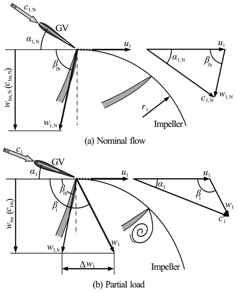
Fig.3 Velocity plans at the impeller inlet for computing the shock loss
The shock loss is then expressed in terms of efficiency loss as Δηshock=Δhshock/H. Based on the geometrical relation presented in Fig.3(b) and by applying the relative velocityw1, the shock loss can be expressed as
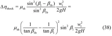
Here, β1brepresents the geometrical blade angle at the impeller inlet. Only when the flow angle1β equals the blade angle β1b, this shock loss vanishes.
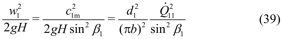
In using of the definition of the unit discharge, the relative velocityw1is further expressible as
For a given flow angle1α in the absolute guide-vanes system, the relative flow angle1β at the impeller inlet is represented as
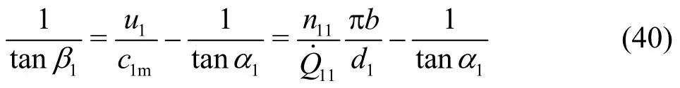
Under the nominal operation condition, one obtains Eq. (6). A fact to be mentioned is that Eq. (40) in its general form also applies to the case of reverse rotation of the impeller, i.e.,n<0.
Equation (38) is finally written as

Except forandn11, all other parameters in this equation are geometrical parameters, which can be considered as given. Obviously, the shock loss does not disappear at=0.
Equation (41) will be used in combination with the swirling loss at the impeller exit to compute the main loss in the Francis turbine for both the partial load and the overload.
1.6.3 Swirling loss at the impeller exit
At partial load or overload, the exit flow out of the impeller possesses a circumferential velocity component. The kinetic energy involved in the related swirling flow will be dissipated in the downstream draft tube and thus must be considered as being lost.The computation of the swirling loss basically relies on integration computations under the consideration of the non-uniform distribution of the circumferential velocity component, which is given by Eq. (33). At the draft tube inlet, the axial flow can be considered to be uniform.
The overall average of the specific kinetic energy,which is involved in the swirling flow at the inlet of the draft tube, is computed through integration of the term, as given by
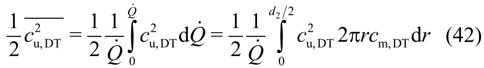
Withand Eq. (33) forcu,DT, this implies
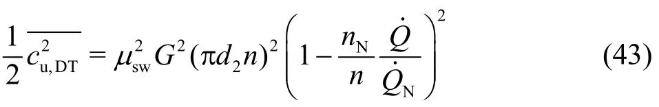
The corresponding efficiency loss is then computed as

With respect to Eq. (1) for the definitions of the characteristic numbersandn11, one finally obtains
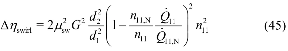
As in Eq. (41), all quantities exceptandn11are known. In addition, the computation according to Eq.(45) is also applicable to the casen<0. Forn=0,the discharge through the impeller is obtained.
It is worth noting that between Eqs. (21) and (43)the following relation can be derived
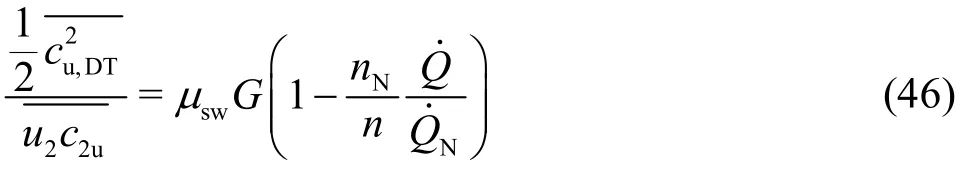
In place ofone can writebecause ofaccording to Section 1.5.
As can also be confirmed there is also

in whichis computed in analogous to Eq. (42).The quantity, however, appears to be less interesting in further computations.
This last equation implies that the kinetic energy,which is involved in the circumferential velocity component, changes along the path from the trailing edge of the impeller blades to the inlet of the draft tube. Because of 2G>1, there is
2. Master equation of the Francis turbine
Based on the computations in Section 1, the master equation of the Francis turbine will be derived in this section.
2.1 Discharge
Combining Eqs. (23) and (34) to collect all partial losses, one obtains, after proper rearrangement

with
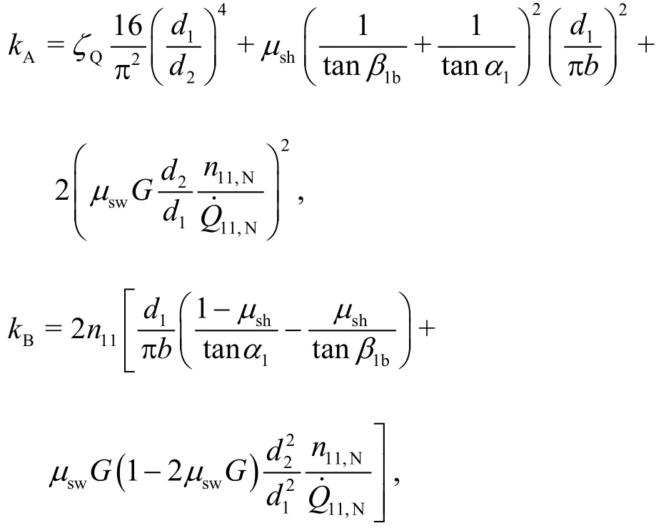
This equation is called the master or main equation of the Francis turbine. It is a simple quadratic polynomial.By solving for the unit dischargefor each given flow angle and unit speed, the characteristics of the Francis turbine can then be obtained in the formThe simple Eq. (48) has been derived b y neglecting the leakage flow. The computations also apply to the case of reverse rotation of the impeller,i.e.,n<0. However, the unit dischargeis generally asymmetrical on both sides ofn11=0. Corresponding computations and comparisons with measurements will be presented below in Section 4.
Atn11=0, it deals with a discharge of the water through the turbine. The unit discharge is obtained in this case as

Because of the composition of the coefficientkA,obviously, the discharge atn=0 is primarily determined by the shock loss at the impeller inlet and the swirling loss at the impeller exit. In the first application of the derived master equation (see Section 4 below), the author sets μsh≈1 and μsw≈ 0.85.
For the nominal setting of the guide vanes(α1,N) and by neglecting the friction-dominant losses(ςQ≈0) as well as for μsh≈1 and μsw≈1, the coefficientkAis simplified, with respect to Eqs. (5)and (6), to
Eq. (49) then becomes
It is directly related to the nominal discharge.
On the other hand, the unit discharge given in Eq.(49) can also be directly obtained from Eq. (41) for the shock loss, Eq. (45) for the swirling loss and Eq.(36) for the flow-dependent friction loss by settingn11=0 and subsequently using Δηshock,0+ Δηswirl,0+ΔηQ=1. Thus, it is clear that the discharge atn11=0 is completely governed by the shock and swirling losses, together with the friction loss. The latter is mostly negligible for partial discharges.
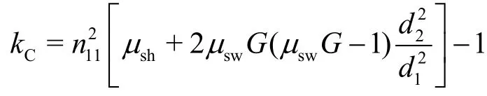
For=0, the unit speed is determined by the coefficientkCfrom Eq. (48), which must vanish in this case, leading to
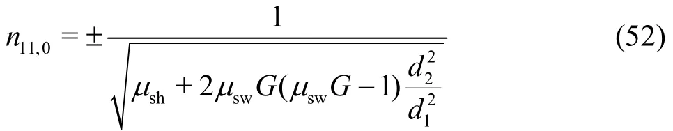
It is basically determined by the diameter ratiod2/d1and the structural constantGand is explicitly independent of the guide vanes angle. With the assumptions of μsh=const , both values (plus and minus) are quasi mirrored. This phenomenon has always been confirmed in practice[2,3], even for pump-turbines. In reality, as also observed in practice,the valuen11,0is a function of the guide vane settings[9,10]. This simply means that μshfor the shock loss at the impeller inlet has to be a function of the guide vane angle, while μswonly considers the exit flow out of the impeller and can thus be assumed to be independent of the guide vane settings. When the influence of the rotational speed on the coefficient μshis also considered, then one can generally write μsh=f(α1,n11). More investigations on this functionality should be completed in the future. As will be shown in Section 4, Eq. (52) also provides a possibility to experimentally determine the coefficient μshunder the condition=0.
2.2 Hydraulic torque and power
In accounting for the hydraulic efficiency, the hydraulic power of the Francis turbine is computed as

The computation of the hydraulic efficiency is referred to Eq. (22) or, equivalently, to Eq. (34).
On the other hand, the hydraulic power is represented as the product of the hydraulic torque exerted on the shaft (momentMhyd) and the angular speed(2πn) of the shaft, as given byPhyd=2πnMhyd. By equalising this equation with Eq. (53) and further by applying Eq. (1), one obtains

In this equation, the unit dischargehas already been computed by Eq. (48).
As mentioned in connection with the hydraulic torque in Section 1.5, the above equation does not apply to the case=0, at which the turbine mode changes to the pump mode and the real torque does not disappear. The pumping effect would takes place[16].
Equation (54) in its given form could not be directly applied to the casen=0. From Eq. (29),however, one obtains immediately
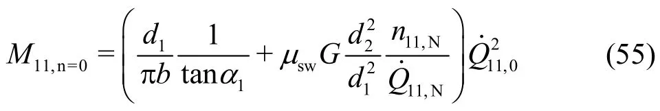
Forrefer to Eq. (49). In Section 4, corresponding computations are compared with measurements.
2.3 Hydraulic efficiency
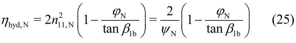
The hydraulic efficiency of the Francis turbine is given, once the discharge has been computed from Eq.(48) and subsequently inserted into Eq. (23). Under nominal operation condition, one obtains with respect to Eq. (1)
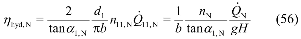
which is equivalent to Eq. (25).
3. Runaway speed of the Francis turbine
After load rejection, the available head and the water flow cause the turbine unit to speed up towards a maximum which is called the runaway speed. This maximum speed behaves as a critical value for the mechanical safety of both the impeller and the rotor of the generator. Because under runaway speed no energy exchange between the flow and the impeller occurs, both the hydraulic efficiency and the torque vanish (ηhyd,R=0,M11,R=0). The runaway speed is,thus, clearly determined. From Eq. (23) or Eq. (29)one firstly obtains
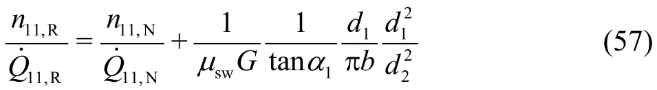
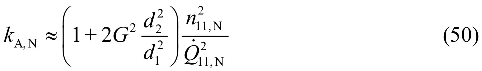
On the other hand, the condition ηhyd,R=0 can also be applied to Eq. (34). Because under the runaway speed the discharge is much smaller than that at the nominal operation point, the term ΔηQfor the friction loss can be neglected for simplicity. Thus, one obtains from Eq. (34) with respective expressions for Δηshockand Δηswirl
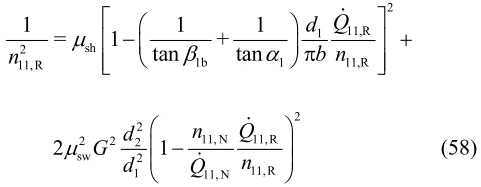
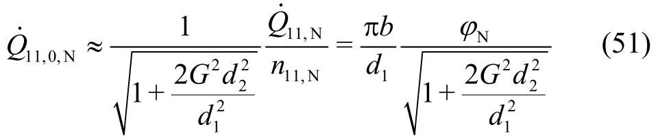
By inserting Eq. (57) into Eq. (58), the unit runaway speed can be computed. Moreover, with Eq. (5) for use ofNφ, one finally obtains for the positive rotational speed

or in the short form
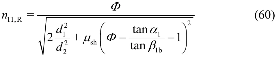
in which the following substitution is used
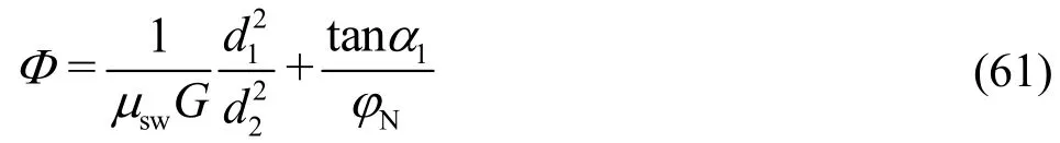
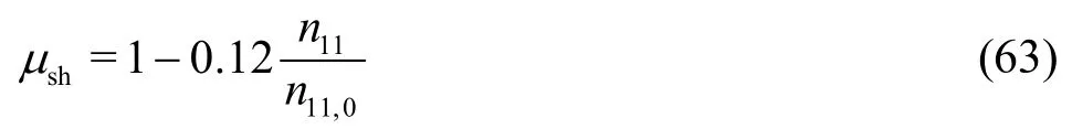
The runaway speed has been shown as a function of the guide vane angle (α1). The coefficient μshcan be set equal to that in Eq. (52), because bothn11,Randn11,0are found in the upper region of the discharge characteristics. In addition, the approximation μsw≈1 can be applied without causing significant inaccuracy, see Section 4 below. Especially for β1b≈ π/2, Eq. (60) can be further simplified because 1/tanβ1b≈0.
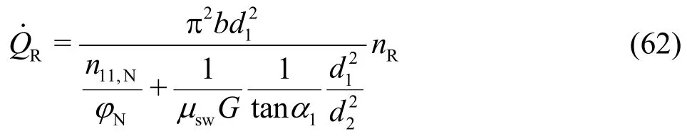
The discharge under the condition of runaway speed is then obtainable from Eq. (57). In the explicit form, this is written, by further using Eq. (5) for φN,as
It should be mentioned that up to now the runaway speed of the Francis turbine has often been given in the form ofnR/nN. In Ref. [17], for instance, the runaway speeds of the Francis turbine have been indicated to benR/nN=1.6-2.2. To the first, this indication is much coarse, since the deviation from the median (1.9) is exceedingly high (±16%). To the second, as can be confirmed from Eq. (60), the rationR/nNis not a representative parameter for Francis turbines with changeable guide vane angles for flow regulations.
4. Application example
In Section 2, the master equation of the Francis turbine has been derived and given by Eq. (48). This equation will now be applied to an existing Francis turbine at the Oberhasli Hydroelectric Power Company (KWO). The characteristics of this turbine in the form of=f(α1,n11)andM11=f(α1,n11)were obtained based on model tests by the company Andritz. The specific speed and the structural constant arenq=38 andG=0.675, respectively.
First, the asymmetric profile of relation=f(α1,n11) is shown in Fig.4. For simplicity, μsh=1 has been assumed for bothn11,0>0 andn11,0<0.

Fig.4 Asymmetric distribution of the discharge as a function of the unit rotational speed Q1 1=f( n 11)
Forn=0, both discharge and hydraulic torque have been given by Eqs. (49) and (55), respectively.With ςQ=2, μsh≈1 and μsw≈ 0.85, corresponding results are shown in Figs. 5, 6. For comparison purposes, the case of μsw=1 has also been shown.Generally, the assumption of μsw=1 does not cause significant computation errors.

Fig.5 Unit discharge at standstill of the turbine, comparison between computations and measurements

Fig.6 Unit torqueat stand still of the turbine,comparison between computations and measurements
As from Eq. (52) for=0, the shock loss coefficient μshhas to be chosen, in order to achieve the valuen11,0which agrees with the measurements.For the Francis turbine currently considered, the author gets μsh≈ 0.88 atn11,0for a middle flow angle.
Then the relation μsh=f(n11)is assumed, for simplicity, to be a linear function
With this assumption and for μsw=0.85, both=f(α1,n11) from Eq. (48) andM11,hyd=f(α1,n11)from Eq. (54) have been computed and compared with measurements, as shown in Figs. 7, 8, respectively.Satisfactory agreement between computations and measurements confirms the applicability of the master equation of the Francis turbine and the related flow mechanical models.

Fig.7 Turbine characteristics (unit discharge) and comparison between computations and measurements for the Francis turbine at the hydro power plant KWO
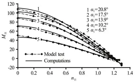
Fig.8 Turbine characteristics (unit torque) and comparison between computations and measurements
The runaway speed and its dependence on the guide vane angles have also been computed according to Eq. (59) and are shown in Fig.7. In this computa-tional example, the runaway speed has been found to benR/nN=1.64-1.70, depending on the guide vane angles. These values are obviously much more accurate than the indication in Ref. [17] withnR/nN=1.6-2.2.
The related discharge, as computed from Eq. (57),can be directly read out from the diagram.
While performing the computations of the turbine characteristics, both the hydraulic efficiency and diverse losses have also been obtained. For the guide vane angles equal to 8.2° and 17.5°, for instance,the computed hydraulic efficiencies are compared with measurements, as shown in Fig.9, again with excellent agreement. The slope of the hydraulic efficiencies atn11=0 is almost constant for all guide vane angles and takes dηhyd/dn11≈ 2. This circumstance has already been the subject in Ref. [4] to reveal the computations as being self-validated.
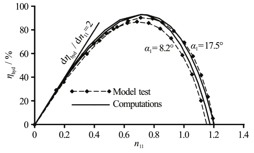
Fig.9 Turbine characteristics (hydraulic efficiencies) and comparison between computations and measurements
In Fig.10(a), both the shock and the swirling losses are shown, which are obtained for the nominal setting of guide vanes (α11,N=17.5°). Obviously, the great deficit in the hydraulic efficiency of the Francis turbine at operations out of the design point(n11,N=0.71) is mainly caused by the shock and the swirling losses.
At other setting angles of guide vanes, as shown in Fig.10(b), both the shock and the swirling losses will never be simultaneously zero. This simply implies that nominal flows can no longer be reached.
5. Conclusions
In order to get the general expressions of the characteristics of Francis turbines, the nominal operation condition of the turbine has been extended to involve the variability of the rotational speed. The operation point of a Francis turbine with given geometric design (impeller diameter and blade profiles) will then be determined by the hydraulic head, the rotational speed and the setting angle of the guide vanes. The determination mechanism among all these design and operation parameters, however, has so far not clearly been revealed. There has actually not been any available computational method which could combine all these parameters with the flow rate, the power output, and the hydraulic efficiency. This lack in the hydraulic computations largely hinders the understanding of the flows in the turbine and hence the attempt of the flow optimization.

Fig.10 Shock and swirling losses of the Francis turbine
For this reason, a computational method has been developed to reveal the hydraulic mechanism in the Francis turbine. The method combines the angular momentum (i.e., Euler) and the energy equations. The latter accounts for all sensible and reasonable losses which occur at the operation points out of the design point. These are shock loss at the impeller inlet, the swirling loss at the impeller exit and the flow dependent frictional losses. The former two losses dominate in influencing the characteristics and the hydraulic efficiency of a Francis turbine. Both together determine the discharge of water through the impeller at the standstill (n=0). The analyses finally lead to the master equation of the Francis turbine,which uniquely combines the geometric design of the impeller with the dynamic operations of the turbine system. It, thus, enables the complete characteristics of the Francis turbine to be determined by computation. This includes not only the discharge, the hydraulic torque and the hydraulic efficiency, but also the runaway speed of the Francis turbine. All computations have been compared with measurements, with excellent agreement. The method of using the master equation of the Francis turbine can, thus, be considered to be self-validated, as designated in Ref. [4].
The operational instability in the upper range of the rotational speed arises from the total flow separation at the impeller inlet and the flow stagnation in the impeller channels. Because the hydraulic efficiency tends to be zero, the computational model shown in this paper reaches its upper limit. A new computational model needs to be worked out in the future.
[1] Drtina P., Sallaberger M. Hydraulic turbines–basic principles and state-of-the-art computational fluid dynamics applications [J].Proceedings of the Institution of Mechanical Engineers Part C Journal of Mechanical Engineering Science, 1999, 213(1): 85-102.
[2] Zeng W., Yang J., Cheng Y. Construction of pump-turbine characteristics at any specific speed by domain-partitioned transformation [J].Journal of Fluids Engineering, 2015,137(3): 031103.
[3] Zeng W., Yang J. D., Cheng Y. G. et al. Formulae for the intersecting curves of pump-turbine characteristic curves with coordinate planes in three-dimensional parameter space [J].Proceedings of the Institution of Mechanical Engineers Part A Journal of Power and Energy, 2015,229(3): 324-336.
[4] Zhang Zh., Titzschkau M. Self-validated calculation of characteristics of a Francis turbine and the mechanism of the S-shape operational instability [J].IOP Conference Series: Earth and Environmental Science, 2012, 15(3):032036
[5] Zhang Zh. Streamline similarity method for flow distributions and shock losses at the impeller inlet of the centrifugal pump [J].Journal of Hydrodynamics, 2018,30(1): 140-152
[6] Hasmatuchi V., Roth S., Botero F. et al. High-speed flow visualization in a pump-turbine under off-design operating conditions [C].25th IAHR Symposium on Hydraulic Machinery and Systems, Timisoara, Romania, 2010.
[7] Staubli T., Senn F., Sallaberger S. Instability of pump turbines during start-up in turbine mode [C].Hydro 2008,Ljubljana, Slovenia, 2008.
[8] Martinm C. Instability of pump-turbines with S-shaped characteristics [C].20th IAHR Symposium on Hydraulic Machinery and Systems, Charlotte, USA, 2000.
[9] Zuo Z., Fan H., Liu S. et al. S-shaped characteristics on the performance curves of pump-turbines in turbine mode–A review [J].Renewable and Sustainable Energy Reviews,2016, 60: 836-851.
[10] Sun H., Xiao R., Liu W. et al. Analysis of S characteristics and pressure pulsations in a pump-turbine with misaligned guide vanes [J].Journal of Fluids Engineering, 2013,135(5): 511011.
[11] Cavazzini G., Covi A., Pavesi G. et al. Analysis of the unstable behavior of a pump-turbine in turbine mode:Fluid-dynamical and spectral characterization of the S-shape characteristic [J].Journal of Fluids Engineering,2016, 138(2): 021105.
[12] Merino J. M., Lopez A. ABB Varspeed generator boosts efficiency and operating flexibility of Hydro power plant[J].Fuel and Energy Abstracts, 1996, 37(4): 272.
[13] Terens L., Schäfer R. Variable speed in Hydro power generation utilizing static frequency converters [C].Proceedings of the International Conference on Hydro power,Nashville, Tennessee, 1993, 1860-1869.
[14] Käling B., Schütte T. Adjustable speed for hydro power applications [C].ASME Joint International Power Generation Conference, Phoenix, Arizona, 1994.
[15] Susan-Resiga R., Ciocan G., Anton I. et al. Analysis of the swirling flow downstream a Francis turbine runner [J].Journal of Fluids Engineering, 2006, 128(1): 177-189.
[16] Nielsen T. K., Olimstad G. Dynamic behaviour of reversible pump-turbines in turbine mode of operation [C]. The 13th International Symposium on Transport Phenomena and Dynamics of Rotating Machinery, Honolulu, USA,2010.
[17] ESHA. Guide on how to develop a small Hydro power plant[R]. European Small Hydro power Association (ESHA),2004.
- 水动力学研究与进展 B辑的其它文章
- Numerical analyses of ventilated cavitation over a 2-D NACA0015 hydrofoil using two turbulence modeling methods *
- Couple stress fluid flow in a rotating channel with peristalsis *
- 2-D eddy resolving simulations of flow past a circular array of cylindrical plant stems *
- Revisit submergence of ice blocks in front of ice cover-an experimental study *
- Energy dissipation of slot-type flip buckets *
- Some notes on numerical simulation and error analyses of the attached turbulent cavitating flow by LES *