
Effect of mesoscale wind stress-SST coupling on the Kuroshio extension jet*
2018-07-11 01:57WEIYanzhou魏艳州ZHANGRonghua张荣华WANGHongna王宏娜KANGXianbiao康贤彪
关键词:荣华
WEI Yanzhou (魏艳州) ZHANG Ronghua (张荣华) WANG Hongna (王宏娜) KANG Xianbiao (康贤彪)
1Key Laboratory of Ocean Circulation and Waves,Institute of Oceanology,Chinese Academy of Sciences,Qingdao 266071,China
2University of Chinese Academy of Sciences,Beijing 100049,China
3Qingdao National Laboratory for Marine Science and Technology,Qingdao 266000,China
4College of Air Traffc Management,Civil Aviation Flight University of China,Guanghan 618307,China
AbstractEffect of mesoscale wind stress-SST coupling on the Kuroshio extension jet is studied using the Regional Ocean Modeling System. The mesoscale wind stress perturbation (τ MS) is diagnostically determined from modelled mesoscale SST perturbation (SSTMS) by using their empirical relationship derived from corresponding observation. From comparing two experiments with and without theτ MSfeedback, it is found that the interactively representedτ MS-SSTMScoupling can modulate the kinetic energy along the Kuroshio extension jet, with little effect on the Kuroshio pathway. Similar results are also obtained in three additional sensitivity experiments, which consider half strength of theτ MS, and the momentum flux and heat flux effect induced byτ MS, respectively. That means simply taking into account theτ MS-SSTMScoupling has little effect on improving the simulation of the Kuroshio Current system.
Keyword:mesoscale wind stress-SST coupling; Kuroshio extension; surface kinetic energy; ocean modeling
1 INTRODUCTION
significant mesoscale coupling perturbations (at a size of 100-1 000 km) in the ocean and atmosphere are observed in the Kuroshio Extension (e.g., Nonaka and Xie, 2003; Xie, 2004; Chelton et al., 2004;Maloney and Chelton, 2006; Small et al., 2008). For instance, the perturbed sea surface temperature (SST)is accompanied with perturbations in air temperature,cloud fraction, wind stress, and sea level pressure(e.g., Nonaka and Xie, 2003; Minobe et al., 2008;Tokinaga et al., 2009; Bryan et al., 2010). Mesoscale perturbations of SST (SSTMS) and sea surface wind stress (τMS) are positively correlated (e.g., Maloney and Chelton, 2006; Bryan et al., 2010; Chelton and Xie, 2010), suggesting that theτMSare driven by the SSTMS, by means of downward momentum transport and pressure adjustment (e.g., Small et al., 2008;Bryan et al., 2010; Frenger et al., 2013).
The mesoscale air-sea coupling has significant effect on both the atmosphere and ocean. On one hand, SST perturbations can directly affect the wind stress divergence and cloud fraction in the atmospheric boundary layer, and are hence important for precipitation simulations (e.g., Minobe et al., 2008;Putrasahan et al., 2013). On the other hand, the induced wind stress perturbations can in turn impact the oceanic conditions in the Kuroshio extension(e.g., Wei et al., 2017). Specifically, they can inhibit the mesoscale SST perturbations by means of surface heat flux and affect the local Ekman upwelling by means of momentum flux (e.g., Nonaka and Xie,2003; Maloney and Chelton, 2006; Chelton, 2013;Wei et al., 2017).
The effect of mesoscale air-sea coupling on the oceanic jet has been previously studied from different methods. Ma et al. (2016) demonstrated that the mesoscale air-sea coupling had an effect ofintensifying the Kuroshio based on the atmosphereocean coupled models. In their work, the effect of mesoscale air-sea coupling was isolated through comparing two experiments with and without the SSTMSbefore being used to force the atmosphere model. Using an idealized high-resolution quasigeostrophic (QG) ocean model, Hogg et al. (2009)demonstrated that the mesoscale wind stress-SST coupling can reduce the strength of the ocean jet.These different results are probably caused by their different experimental settings. For instance, only the effect ofτMS-SSTMScoupling is considered by Hogg et al. (2009), while all the atmospheric responses to SSTMSare taken into account by Ma et al. (2016).Thus, there are uncertainties in the effects of mesoscale air-sea coupling.
In Wei et al. (2017), we took a simple approach to incorporate theτMS-SSTMScoupling in the ocean model to study its effect on the oceanic conditions in the Kuroshio extension. This study continues to examine the effect ofcoupling on the Kuroshio extension jet.
2 METHODOLOGY
2.1 Ocean model
The Regional Ocean Modeling System (ROMS) is employed to assess the effect ofcoupling on the Kuroshio extension jet. The ROMS is a threedimensional, hydrostatic, free-surface, terrainfollowing numerical model (e.g., Shchepetkin and McWilliams, 2005). The model domain is from 20°S to 60°N in latitude and from 100°E to 70°W in longitude. Longitude resolution is 1/8°, and latitude resolution is 1/8°×cos (latitude), with 50 s-coordinate levels in the vertical direction. The temperature,salinity, velocity, and surface elevation at boundaries are prescribed by spatial interpolation of the WOA2009 datasets. The 3D velocity, temperature,and salinity are nudged to boundary values at these three open lateral boundaries with a 360-day time scale for outf l ow and 3-day for inf l ow. The logical switches of nudging/relaxation are also turned on to nudge the 2D momentum and 3D temperature fi elds to their climatology with a 360-day time scale. The time steps are 30 s and 300 s for the 2-D and 3-Dequations. At each time step, the surface net heat flux sensitivity to SST (dQ/dSST) is calculated and used to introduce thermal feedback to correct net surface heat flux (Barnier et al., 1995). More detailed descriptions of the model settings are given in Wei et al. (2017). After 20 year integration, a quasiequilibrium state is obtained; and the derived oceanic variables in that time are used as initial conditions for experiments as described below.

Table 1 τMS-induced heat flux and momentum flux effects considered in five experiments
2.2 Numerical experiments
In order to assess the effect ofτMS-SSTMScoupling,two experiments with and without theτMSfeedback are carried out. In no-feedback experiment, the model settings are as normal. In the feedback experiment,theτMS-SSTMScoupling is incorporated in the model in the Kuroshio extension region.
TheτMS-SSTMScoupling is incorporated into the ocean model by interactively determining theτMSfrom SSTMSfollowing their close relationship.τMSis estimated from the equation:τMS=a×SSTMS, whereais regression coeffcient and is taken 0.01 (Wei et al.,2017). The SSTMSsimulated by the ocean model is isolated by using the locally weighted regression(loess) method (e.g., Cleveland and Devlin, 1988). In this study, a 10° latitude ×30° longitude loess spatial high-pass fi lter is used (Wei et al., 2017). The derivedτMSis then used to combine with the climatology wind stress to force the ocean in the feedback experiment,with the amplitude changed from |τ| to |τ|+τMS, and the wind directionθunchanged. The area where theτMSSSTMScoupling is considered is located east of Japan,because theτMSand SSTMSare observed to be active there.
TheτMSacts to impact the ocean by means of surface momentum flux and heat flux. In order to examine the sensitivity of the results toτMSand understand the way by whichτMSimpacts the ocean,three additional experiments are carried out. They are half-feedback experiment (which uses half strength ofτMS), HF-feedback (τMSis allowed to inf l uence the surface heat flux only) and MF-feedback (τMSis allowed to inf l uence the surface momentum flux only)experiments (Table 1). In order to enhance computational speed,τMSis updated daily instead ofinstantly in all the above experiments. All the experiments are run for 10 years with monthly averaged output.
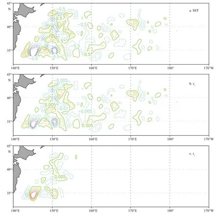
Fig.1 A snapshot of the SSTMS(unit: °C) simulated by the ocean model (a), and the zonal (b) and meridional (c) wind stress perturbations (unit: N/m2) derived from it
3 RESULT
3.1 The effectiveness of the empirical coupling
The high resolution model based on ROMS is eddy-permitting, even though wind stress forcing is climatology. As shown in Fig.1a, the simulated SSTMShas a size of about 100-400 km and an amplitude of about 2.5°C, which agree with that found in satellite observation (e.g., Wei et al., 2017). Figure 1b and c show the zonal and meridional mesoscale wind stress perturbations derived from the SSTMS. The spatial distribution of zonal wind stress perturbations agrees with that of SSTMS. The wind stress fi eld perturbations are northwesterly in the area of positive SSTMSwhile southeasterly in the area of negative SSTMS, with the magnitude at about 0.03 N/m2. Therefore, the mesoscale wind stress fi eld perturbations can be derived from the empirical relationship with respect to SSTMS.

Fig.2 Correlation coeffcients between SSTMSand τMSin no-feedback (a) and feedback (b) experiments Contour interval is 0.1, with small value (<0.4) contours omitted.
Positive correlation betweenτMSand SSTMSis obtained after incorporation of theτMS-SSTMScoupling(Fig.2). Correlation coeffcient betweenτMSand SSTMSwas often simulated incorrectly in the low resolution climate models (e.g., Maloney and Chelton,2006; Bryan et al., 2010). This problem exists in the no-feedback experiment when theτMSis not incorporated into the ocean model (Fig.2a). The incorporation of the empiricalτMS-SSTMScoupling helps to improve this problem, and enhances the correlation between them (Fig.2b). These results altogether suggest that the empiricalτMS-SSTMScoupling utilized here is effective to capture their inherent relationship.
3.2 Effect on the Kuroshio extension jet
TheτMS-SSTMScoupling is interactively incorporated into the model to represent theτMSfeedback on the ocean. In this subsection, the effect ofτMSon the Kuroshio extension jet is isolated through comparing two experiments with and without it.Figure 3a and b show the mean kinetic energy simulated by no-feedback and feedback experiments as averaged from year 21 to 30. The kinetic energy can reach 2.0 m2/s2, suggesting that the Kuroshio velocity can reach 1.4 m/s. significant kinetic energy difference between two experiments is seen along the Kuroshio extension jet (Fig.3c); the largest difference exceeds 0.2 m2/s2, which is about 10% of the mean kinetic energy.
Figure 3d-f show corresponding distance-depth cross-sections of zonal velocities simulated by nofeedback and feedback experiments averaged from 142°E to 152°E, and their difference. It is seen that the Kuroshio Current can reach to a depth of 1 500 m,with relatively weak counter current on its two fl anks(Fig.3d). The position of the Kuroshio extension jet is almost unchanged compared with that in the nofeedback experiment (Fig.3e). The velocity difference between no-feedback and feedback experiments is negative at the Kuroshio axis, while positive at its two sides (Fig.3f). The difference with the same sign can reach to a depth of 2 000 m. These results suggest that theτMS-SSTMScoupling can modulate the Kuroshio velocity, while has little effect on the position of the Kuroshio pathway (Fig.3d and e).
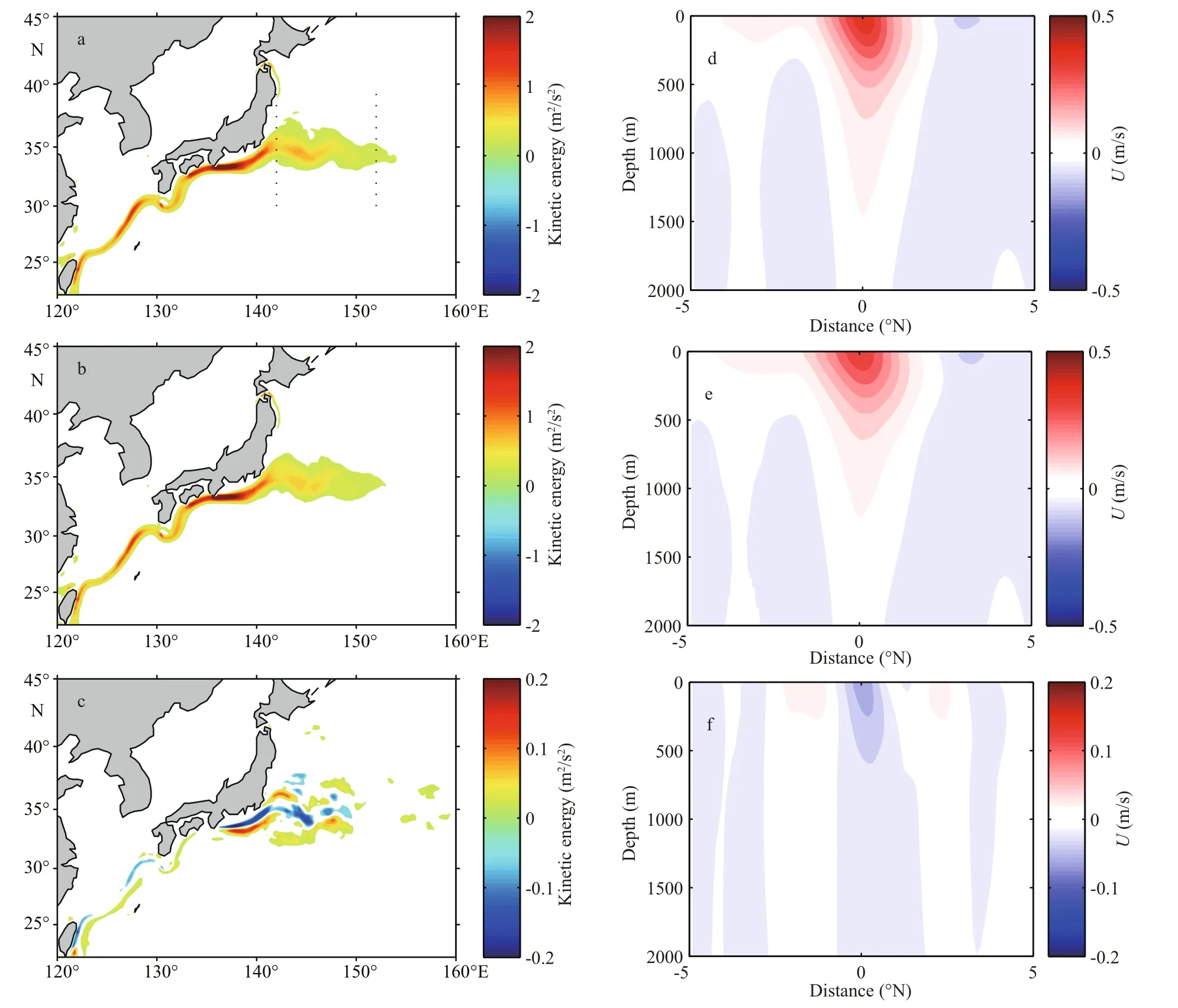
Fig.3 The surface kinetic energy (unit: m2/s2) simulated in no-feedback (a) and feedback (b) experiments, and their difference(c); the corresponding zonal velocity (unit: m/s) averaged from 142°E to 152°E are shown in (d), (e), and (f)Thexaxis in d-f denotes the distance from the Kuroshio axis (0), with negative (positive) values indicating distances north (south) of the Kuroshio jet. All results are averaged from the model year 21 to 30.
The kinetic energy differences in half-feedback,MF-feedback and HF-feedback experiments relative to that in the no-feedback experiment are shown in Fig.4. It is seen that the kinetic energy has substantial changes along the Kuroshio extension jet in these experiments. The results suggest that theτMS-SSTMScoupling acts to affect the Kuroshio surface kinetic energy through either the way of moment flux or heat flux. However, the position of the Kuroshio extension jet is not found to change systematically in these experiments. It can be also found that the magnitude of surface kinetic energy difference in the halffeedback experiment (Fig.4a) is not significantly reduced relative to that in the feedback experiment(Fig.3c), suggesting that the kinetic energy difference might be not linearly related to the strength ofτMS.Moreover, the surface kinetic energy difference in the feedback experiment (Fig.3c) seems to be not a simple combination of the differences caused respectively by the effects of surface heat flux and momentum flux(Fig.4b and c).
The effects ofτMS-SSTMScoupling are also seen in the SST, wind stress curl and surface heat flux. Figure 5a shows the SST difference between no-feedback and feedback experiments as averaged over the model year 21-30. It is seen that the SST difference can reach 0.3°C, but in a structure that is very patchy.Figure 5b shows the wind stress curl difference between two experiments. The difference in wind stress curl between the two experiments is about 0.5×10⁻⁷N/m3, which is a small portion (about 10%)relative to the observed mesoscale wind stress curl perturbations (e.g., Wei et al., 2017). Figure 5c shows the surface net heat flux (downward positive)difference between the two experiments, which has a magnitude of about 15 W/m2.
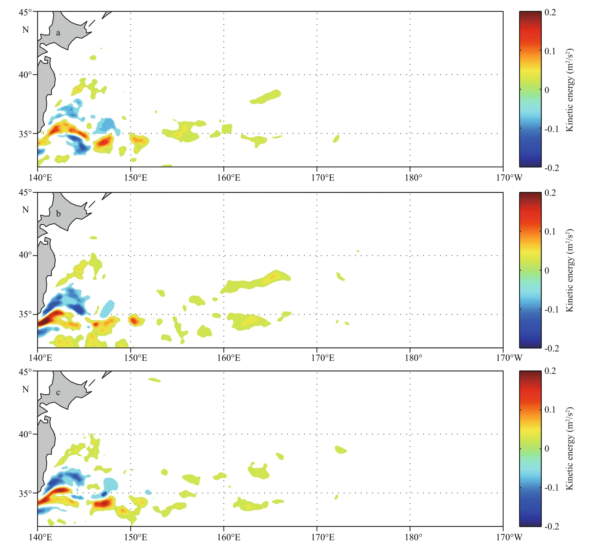
Fig.4 The surface kinetic energy differences (relative to no-feedback experiment) in half-feedback (a), MF-feedback (b) and HF-feedback (c) experiments averaged from the model year 21 to 30
An interesting phenomenon is that theτMSinduced kinetic energy difference is small east of 150°E(Fig.3c), although there are large surface net heat flux,SST, and wind stress curl differences (Fig.5). That means the kinetic energy difference is not simply caused by the differences of these three terms. As the Kuroshio speed is large, a small change in the Kuroshio extension jet (e.g., intrinsic fluctuations)might results in large difference in the surface kinetic energy. For instance, the wind stress curl induced Ekman pumping might interact with the Kuroshio and result in the distinct kinetic energy difference along the Kuroshio pathway.
4 CONCLUDING REMARKS
The effect of mesoscale wind stress-SST coupling on the Kuroshio extension jet is investigated by using a high resolution ocean model. The perturbed sea surface wind stress fi eld is estimated empirically from modeled SSTMSand then incorporated into the ocean model. The effect ofτMS-SSTMScoupling on the Kuroshio extension jet is isolated through comparing two experiments with and without this effect. It is found that thecoupling can substantially affect the surface kinetic energy along the Kuroshio extension jet, with little effect on the climatology mean position of the Kuroshio pathway. Further sensitivity analyses suggest that theτMScan affect the surface kinetic energy from either the way of surface heat flux or momentum flux. The interactively representedτMS-SSTMScoupling also affects the climatology mean SST, wind stress curl and surface heat flux, but the induced differences are all very patchy.

Fig.5 SST (a), wind stress curl (b) and surface heat flux (c) differences between no-feedback and feedback experiments as averaged from year 21 to 30Positive curl value indicates upwelling, while negative value indicates downwelling. Surface heat flux is negative while the ocean loses heat.
Hogg et al. (2009) pointed out that theτMS-SSTMScoupling can reduce the strength of the ocean jet using a high-resolution quasigeostrophic ocean model. Ma et al. (2016) pointed out that the mesoscale air-sea coupling can enhance the strength of the Kuroshio extension jet and affect the position of the Kuroshio axis. These different results arise from different models and ways used to isolate the effect of mesoscale air-sea coupling. Hogg et al. (2009)examined the effect ofτMS-SSTMScoupling from an idealized ocean model. Ma et al. (2016) isolated the effect of mesoscale air-sea coupling by utilizing the atmosphere-ocean coupled models, by comparing two experiments with and without the SSTMScomponent before being provided to the atmosphere model. The approach used by Ma et al. (2016) is advantageous over many aspects; however, the induced large scale atmospheric changes might also interface in their results. In relative, our current study isolated the effect ofτMS-SSTMScoupling in a cleaner way. This study demonstrates that the kinetic energy difference between no-feedback and feedback experiments is large in vicinity of the Kuroshio, which might be linked to interactions between small scale oceanic disturbances and the Kuroshio. This study shows that there is no change in the Kuroshio pathway(Fig.3a and b) after incorporation ofτMS-SSTMScoupling.
The results derived in this study have some implications on the climate model biases. The long term mean SST difference induced byτMSis patchy(Fig.5a), so that it could not account for the systematic SST biases appeared in climate models. Moreover,theτMS-SSTMScoupling is not found to affect the position of the long term mean Kuroshio extension jet, so that it has little effect on improving the simulations of the Kuroshio Current system.
猜你喜欢
中国典型病例大全(2022年9期)2022-04-19
汽车维修与保养(2021年8期)2021-02-16
音乐天地(音乐创作版)(2020年8期)2020-11-05
艺术品鉴(2020年9期)2020-10-28
汽车维修与保养(2020年11期)2020-06-09
疯狂英语·新阅版(2019年11期)2019-09-10
造纸信息(2019年7期)2019-09-10
蓝盾(2018年10期)2018-11-05
作文周刊·小学一年级版(2016年32期)2017-03-02
作文周刊·小学一年级版(2016年32期)2017-03-02
 Journal of Oceanology and Limnology2018年3期
- Journal of Oceanology and Limnology的其它文章
- Response of the North Pacific Oscillation to global warming in the models of the Intergovernmental Panel on Climate Change Fourth Assessment Report*
- Surface diurnal warming in the East China Sea derived from satellite remote sensing*
- Cross-shelf transport induced by coastal trapped waves along the coast of East China Sea*
- Observations of near-inertial waves induced by parametric subharmonic instability*
- Seasonal variation and modal content ofinternal tides in the northern South China Sea*
- Wave-current interaction during Typhoon Nuri (2008) and Hagupit (2008): an application of the coupled ocean-wave modeling system in the northern South China Sea*