
Convection: a neglected pathway for downward transfer of wind energy in the oceanic mixed layer*
2018-08-02 02:50ZHANGYu张钰WANGWei王伟
关键词:王伟
ZHANG Yu (张钰), WANG Wei (王伟)
Physical Oceanography Laboratory/CIMST, Ocean University of China and Qingdao National Laboratory for Marine Science and Technology, Qingdao 266071, China
Abstract Upper-ocean turbulent mixing plays a vital role in mediating air-sea fluxes and determining mixed-layer properties, but its energy source, especially that near the base of the mixed layer, remains unclear. Here we report a potentially signi ficant yet rarely discussed pathway to turbulent mixing in the convective mixed layer. During convection, as surface fluid drops rapidly in the form of convective plumes,intense turbulence kinetic energy (TKE) generated via surface processes such as wave breaking is advected downward, enhancing TKE and mixing through the layer. The related power, when integrated over the global ocean except near the surface where the direct effect of breaking waves dominates, is estimated at
Keyword: convective mixed layer; convecting plumes; turbulent kinetic energy (TKE); wind energy;surface waves
1 INTRODUCTION
Turbulent mixing in the oceanic mixed layer is very important to circulation and climate. It regulates fluxes across the air-sea interface, facilitates the takeup of excessive heat and CO2from the atmosphere,and more importantly affects properties of water masses that greatly contribute to the large-scale transport of climatically important tracers in the ocean interior (Macdonald and Wunsch, 1996; Sloyan and Rintoul, 2001a, b; Sabine et al., 2004). Formation of various water masses through processes like subduction or deep convection, takes place within the mixed layer and near its base, so turbulent mixing in the deeper part of the mixed layer is of critical importance to water mass properties and hence the Meridional Overturning Circulation. Despite its signi ficance, progress in understanding the mixedlayer turbulent mixing has been relatively slow(D’Asaro, 2014). One of the fundamental questions,the energy source of mixing in the mixed layer,especially near its base, remains unclear, severely impairing our ability to properly represent the related processes in numerical models and predict changes of climate in the future (Iudicone et al., 2008; Cerovečki et al., 2013).
For many decades the dominant paradigm of the upper ocean turbulent mixing consists of three paths(Thorpe, 2005). The first one is the generation of turbulent kinetic energy (TKE) from instability of wind-driven shear, in association with the classical logarithmic boundary layer obeying “the law of the wall”. The second one is the TKE generation at the cost of potential energy in the process of convective instability. The third path is linked to surface gravity waves. Upon generation, they receive most of the wind energy input to the ocean (60 out of 63 TW(1 TW=1012TW), (Wang and Huang, 2004)), and transfer most of the energy to TKE via breaking.Considering that maintaining the deep circulation requires only about 2–3 TW of power (Wunsch and Ferrari, 2004), the ocean circulation would be affected if only a small fraction of the TKE could somehow escape from the surface entering the ocean interior.However according to the conventional understanding TKE generated through wave breaking is concentrated near the surface, declining rapidly downward and approaching the classical “wall-law” scaling within only a few signi ficant wave heights. In this regard, the ocean surface is a large reservoir of TKE that is untapped.
In the past few decades, two mechanisms by which surface wave energy is converted to TKE have been proposed. One is Langmuir circulation which is closely related to Stokes drift of surface waves and is capable of rapidly moving fluid vertically, thereby enhancing turbulence (Langmuir, 1938; Leibovich,1980; McWilliams et al., 1997; Thorpe, 2004).However its maximum effect is well above the base of the boundary layer. The other one is the interaction between non-breaking waves and turbulence, which is argued to be able to greatly improve global model performance (Huang and Qiao, 2010), but its validation and effect are under debate (Kantha et al.,2014). What we discuss here is a “non-local” transport mechanism, that is, strong TKE generated near the surface is carried downward and redistributed through the layer by sinking convective plumes during convection. We begin with a brief discussion of oceanic convective boundary layer in Section 2. The mechanism is discussed with a simple analytical model in Section 3; conclusions are given in Section 4.
2 A RECONSIDERATION OF THE OCEANIC CONVECTIVE BOUNDARY LAYER
Convection is a process whereby surface water parcels undergoing buoyancy loss become dense enough to sink to a depth dependent on local strati fication. The sinking motion is in the form of convective plumes (Thorpe, 2005), converting potential energy to small-scale turbulence, a process that has long been recognized as one major path to turbulent mixing in the oceanic convective boundary(CBL hereinafter) layer, along with other ways such as shear production.
In numerical models, turbulent properties of both the atmospheric and oceanic boundary layers are usually represented by the TKE equation, which describes the budget of TKE (Stull, 1988; Burchard,2002). For the oceanic CBL, we can write the equation as follows (Endoh et al., 2014):
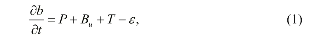
where the time dependency of TKE, which is denoted by b, is related to the production of shear, P, to the production by buoyancy, Bu, to a term T that collectively represents effects of TKE transport, and to the dissipation rate of TKE, ε. Usually, it is assumed that the steady-state TKE is balanced “locally”between source terms, P and Bu, and the sink term, ε(Osborn, 1980; Anis and Moum, 1994). For strongly convecting boundary layer, one would naturally expect a close balance between the buoyancy generation and dissipation. However, as shown by a recent observational study of TKE budget in the oceanic CBL (Endoh et al., 2014), the generation by buoyancy is relevant in the upper part of the layer, but declines quickly downward and becomes a sink,rather than a source of TKE, in the lower half of the layer. The shear generation term, though comparable with Bunear the surface, decays quickly downward as well, being small and positive in the large portion of the layer. Meanwhile, the dissipation rate, estimated by the use of the microstructure data, shows a more or less uniform distribution through the layer. Obviously it is the transport term, T, that dominates the TKE budget in at least the deeper part of the layer, implying that the “local” assumption is not proper. Actually, the similar conclusion has been obtained by both observational studies for the atmospheric CBL and studies of large eddy simulations (Lenschow, 1974;Moeng and Sullivan, 1994; Mironov et al., 2000), but the mechanism behind remains unsettled.
Here we propose a transport mechanism that is related to the downward motion of convective plumes.The convective plumes can have strong vertical velocities, as large as about 0.01 m/s in nighttime mixed layer (Shay and Gregg, 1984) and 0.1 m/s in open ocean convection events (Marshall and Schott,1999). It is thus worth noting that as dense surface water parcels drop, they carry along not only heat, salt and other passive tracers but also their kinematic properties, i.e., the TKE generated via processes such as wave breaking at the surface or Langmuir Cell at intermediate depth. The mechanism, which has been long overlooked, and its effects on turbulent mixing will be discussed with a simple model in following sections.
3 A MODIFIED TURBULENCE MODEL FOR THE OCEANIC CONVECTIVE BOUNDARY LAYER
Convection occurring in the upper ocean is a complicated process in fluenced by many factors. As suggested by rather limited observations in the ocean or in the lab, a convective patch usually consists of multiple convective plumes. The vertical velocity is big and negative within each plume, but weak and positive between plumes. While sinking, plumes entrain and mix with the external fluid, changing density as they go and being strongly in fluenced by rotation of the earth.
We simplify the actual convection process by ignoring mass exchanges with the surrounding fluid while plumes sink and ignoring energy sources of TKE other than wave breaking at the surface. By assuming the related dynamics is axisymmetric about the vertical axis of the convective plume (Fig.1), we consider a two-dimensional “cell” consisting of two limbs: a downward limb composed of downwelling parcels carrying intense TKE in the plume, and an upward limb consisting of slowly upwelling parcels carrying little TKE outside the plume. The two limbs are connected within two very thin sub-layers near the top and the bottom of the mixed layer, where horizontal convergence/divergence occurs to balance vertical motion.
Since TKE is negligible outside plumes, only its distribution inside the plume is of interest. For dynamics in the interior and outside the top and bottom sub-layers, we consider a classical, one dimensional, second-order turbulence closure model(Mellor and Yamada, 1974, 1982; Craig and Banner,1994), which has been widely used in studies of the mixed-layer turbulence and incorporated into general circulation models of ocean and atmosphere.
Here we further simplify the model by only considering the quasi-equilibrium state and modify it by adding an extra term representing vertical advection:

where b is TKE and w is the vertical velocity of sinking plumes and is prescribed for simplicity as a constant of depth, q the turbulent velocity ( b= q2/2), l the turbulent length scale, Sqand B are empirical constants, and the product lqSqrepresents eddy diffusivity. The second term in Eq.2 represents vertical diffusion of energy whereas the final term is the TKE dissipation rate, ε.
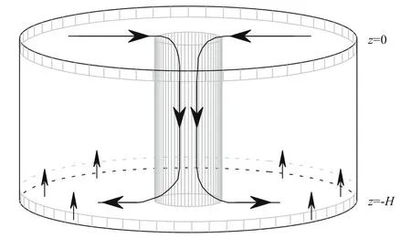
Fig.1 Schematic of a cylindrical “cell” consisting of a convecting plume at the center and upward compensating motion outside
Rather than a “bilinear” form including both the top and bottom boundaries (Craig and Banner, 1994),l( z) is instead assumed to be simply a linear function of depth,

where κ is von Kámán’s constant and z0is the roughness length.
At the surface and the base of the mixed layer we employ the following boundary conditions,
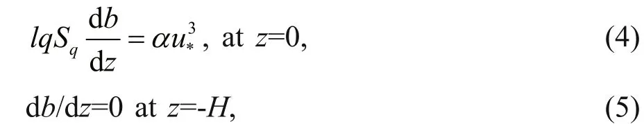
where α is referred to as the “wave energy factor” and u*is the oceanic friction velocity. The former is found quite insensitive to sea state while the latter is closely related to the strength of surface wind stress. The two boundary conditions represent respectively the energy input from breaking waves at the surface and zero flux of energy at the bottom.
It is important to note that the model described above is for the interior of the plume excluding the two sub-layers near the top and bottom of the layer.Therefore, budgets for mass or energy cannot be closed by only considering Eqs.2–5. For example,integrating Eq.1 through the layer and using boundary conditions lead to a budget of the total TKE dissipation:
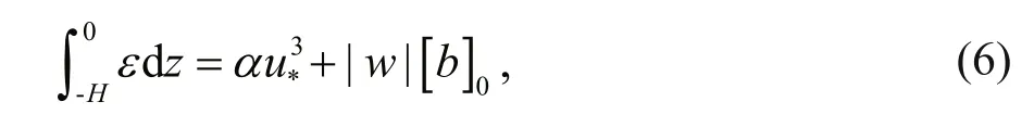

Fig.2 Vertical structure of the dissipation rate, ε, for different magnitude of vertical velocity
where [ b]0denotes the value of b at the surface and its value at the bottom has been ignored. What is basically suggested by Eq.6 is that in addition to TKE induced by wave breaking directly on top of the sinking plume,an extra source term, | w|[ b]0, arises as surface water parcels at nearby horizontal locations converge to compensate for the local sinking motion, and contributes to the turbulence budget of the plume. In this sense, the surface convergence induced by convective sinking makes it possible for the non-local source to enhance the TKE dissipation.
To solve the nonlinear Eqs.2–5, we use the shooting method (see Appendix) with values of those parameters, Sq, B, α, κ, and z0fixed as in Craig and Banner (1994).
As the result of the balance between advection,diffusion, and dissipation, the TKE dissipation rate is large near the surface and decays quickly downward,but the decay tendency is drastically abated with the strengthening sinking motion (Fig.2), suggesting its homogenization or redistribution effect on TKE. In addition, the overall magnitude of TKE through the layer is enhanced by advection, as suggested by Eq.6,and its value at deeper mixed layer is increased by more than five orders as | w| increases from 0 to 0.1 m/s. For mixed layers driven by intermediate to strong convection, the dissipation rate could be as large as 10-7W/kg at the base of the layer, roughly two orders of magnitude higher than that usually found in the seasonal pycnocline.
Turbulence measurements in the upper-ocean have been very scarce, limiting progress of understanding and modeling of convection. As suggested by a few available vertical pro files obtained in the oceanic convective boundary layer, TKE dissipation rate is almost vertically homogeneous (Shay and Gregg,1984; Lombardo and Gregg, 1989), a feature also found prominent in the atmospheric convective boundary layer, except near the sea surface where effects of other processes such as wave breaking are dominant (Anis and Moum, 1995; Noh et al., 2004).The first direct turbulence measurements in oceanic convective boundary layer was made in 1983 (Shay and Gregg, 1984), along which detailed measurements of both atmospheric forcing, including the work of surface wind stress, Ew, and buoyancy flux, Jb0, and boundary layer pro files of temperature, salinity, and velocity, were also obtained, providing a good opportunity to test results of our simpli fied turbulence model (see Appendix).
The friction velocity is readily obtained from measurements of Ew. As to the vertical velocity, we adopt the result of scaling argument, w= a( Jb0H)1/3,where “ a” is a coefficient of proportionality. Few values of “ a” existing in the literature, for example,0.52 was once chosen in a study of deep convection in the Labrador Sea (Steffen and D’Asaro, 2002). Using u*, w, and H as model input, we obtain three curves of TKE dissipation rate and plot them on top of observations. Obviously, model results and observations agree well to each other. Though the highly simpli fied model lacks many elements such as time dependency, generation of turbulence by buoyancy, shear instability or Langmuir circulation,and proper treatment of the two sub-layers, it successfully captured the uniform distribution of TKE with depth. In contrast, model estimates without vertical transport (black lines in Fig.3) are far less than observed values, and decay much more quickly with depth.
The model is further applied to the globe using observations and reanalysis data of air-sea fluxes and mixed layer depth (see Appendix). First of all, the sinking velocity of plumes, estimated as ( Jb0H)1/3, in the convective mixed layer of September is as high as a few cm/s over large regions in the Southern Hemisphere especially along the Antarctic Circumpolar Current (ACC) (Fig.4c), indicative of potential relevance of the proposed mechanism.Distributions of strong convection show similar spatial patterns to that of strong surface wind stress(Fig.4a), yielding large values of the dissipation rate through the mixed layer as a consequence of downward advection of TKE (Fig.4d, e).
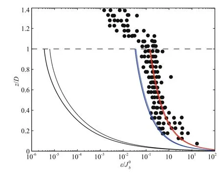
Fig.3 Comparison of TKE dissipation rate between observations (black dots) and model results (solid lines)
To have a general idea of the pattern and magnitude of mixing, we tentatively translate ε at the mixed layer base into a turbulent mixing rate, κv, using the Osborn relation (Osborn, 1980) (Fig.4f). All quantities in Fig.4 show similar patterns, and the most remarkable feature is a yellow-red band extending quasi-zonally in the ACC. In the austral (Southern Hemisphere)winter, the ACC region is characterized with strong westerlies, and intensi fied surface buoyancy loss (not shown), both of which help to generate excessively deep mixed layer over a few hundred meters in many regions. Presumably through downward motion during convection, strong TKE is carried downward from the surface, sustaining enhanced mixing through the entire layer with the amplitude as large as 10-1m2/s.Noteworthily, the area with maximum turbulent mixing is roughly coalesced with regions of mode water distributions such as the Subtropical Mode Water and Subantarctic Mode Water (Siedler et al.,2001), implying the potential signi ficance of the turbulent mixing to the formation/transformation of water masses. As deep winter mixed layer shoals in the austral spring, the strong mixing near the base of the mixed layer may exert an important in fluence on diffusion of mode water located just below.
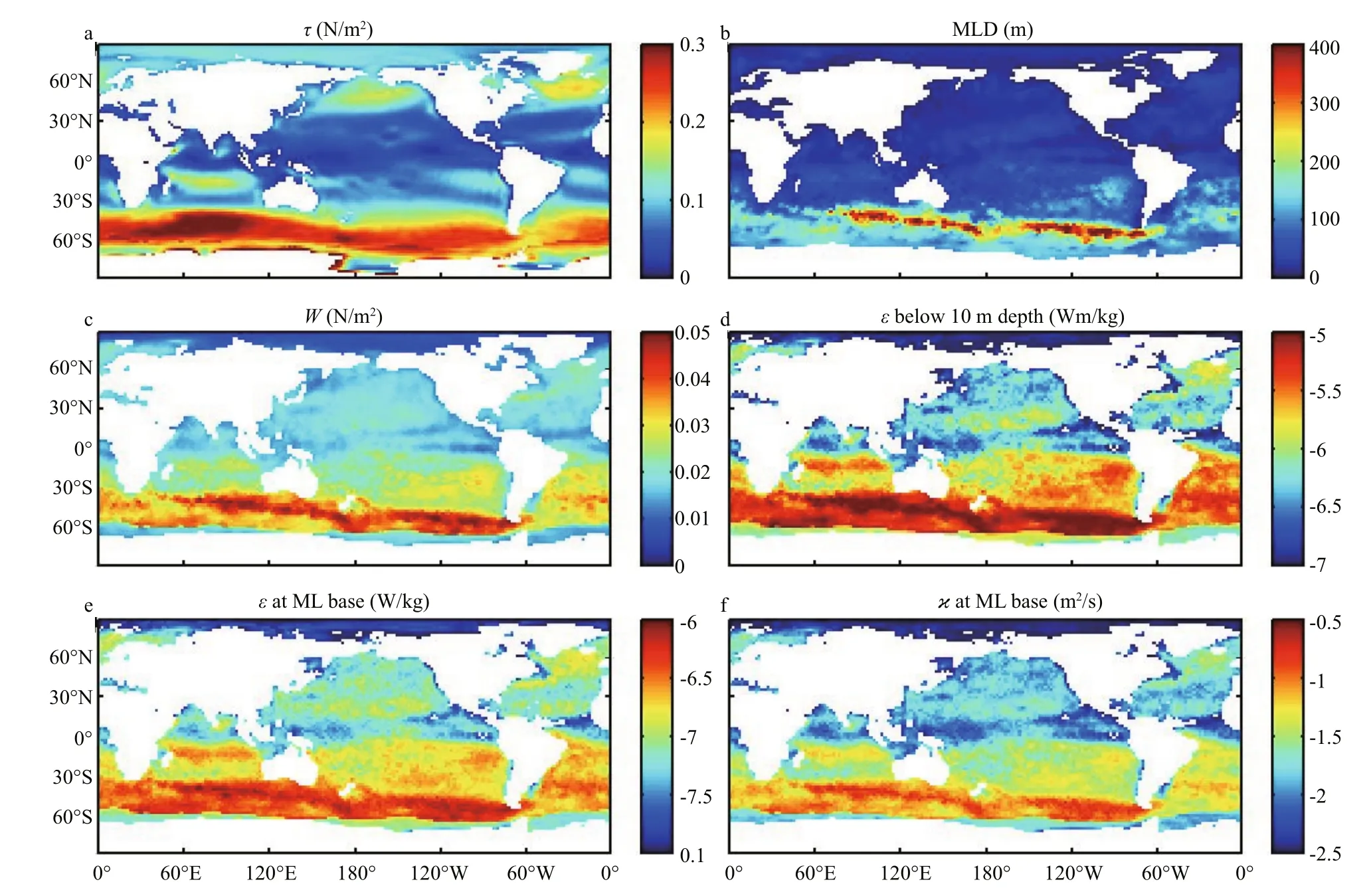
Fig.4 Distribution of TKE dissipation rate and mixing coefficient in September
When integrated globally from the mixed layer base to the 10-m depth, above which the direct effect of breaking surface waves is presumably dominant,the resultant TKE dissipation is about 0.7 TW, over 1% of the total power from wind to surface waves which is, according to our calculation, about 52 TW.Since only monthly climatology for mixed-layer depth is used in above estimates, strength of convection is probably compromised, so is the estimate of the sinking velocity. Hence there is a good reason to expect that the real ratio is probably even higher than what is obtained.
4 CONCLUSION
As demonstrated by both observational and numerical studies, the assumption of a “local”equilibrium of TKE budget for the oceanic or atmospheric CBL is not appropriate and transport of TKE can be relevant, especially in the lower half of the layer. We propose here a potentially important mechanism whereby TKE is redistributed and enhanced in the oceanic convective boundary layer.By sinking convective plumes, intense TKE generated near the surface through processes such as wave breaking can be brought downward to enhance mixing in the middle and deeper mixed layer. Signi ficance of the mechanism was veri fied and evaluated by comparison between in-situ turbulence measurements and results of the widely used one-dimensional Mellor-Yamada second-order turbulence model with an extra term representing the downward advection of TKE by convecting plumes. Applying the model to the global ocean, we found the mechanism is potentially important for water mass properties during its formation/transformation process. By inducing entrainment from below the mixed layer, it may also cause diffusion of mode water, a problem that has attracted much attention in recent years (Oka and Qiu,2012). On the other hand, through the mechanism wind effect reaches great depth of the ocean, especially in regions of open-ocean convection, thus impacting deep ocean circulation.
In spite of its relevance for ocean and climate, the proposed mechanism has long been overlooked and our consideration in this paper is only the first step toward a proper understanding of the process. It is important to note that the applicability of our idealized model can be affected by its assumptions. As pointed out by one reviewer, the linear assumption of the turbulent length scale as a function of depth could lead to questionably large values in deep mixed layer.Some studies also suggested the importance of accounting for the effect of density strati fication in estimating the length scale around the base of the mixed layer (Galperin et al., 1988, 1989; Furuichi and Hibiya, 2015). Further studies are expected to more thoroughly investigate effects of convection in downward transport of surface TKE to the deeper area. For example, the numerical approach using large eddy simulation models (Harcourt, 2013, 2015;Furuichi and Hibiya, 2015) may help us elucidate important issues such as the relation between the local generation of TKE by buoyancy and its non-local advection by convective plumes, the spatial structure and temporal evolution of vertical velocity in the convective mixed layer, and the relative importance of the mechanism compared with other processes that may also induce vertical transport of TKE. Answering these questions can eventually help to improve parameterization of upper-ocean turbulent mixing,and improve our ability to accurately predict climate variation in the future.
5 DATA AVAILABILITY STATEMENT
The sources of the data involved in this paper are contained in the Appendix.
6 ACKNOWLEDGEMENT
The authors would like to thank the anonymous reviewers for their valuable suggestions.
APPENDIX
1 Solution of the turbulence model
Following Craig and Banner (1994), we assume l is a linear function of depth:

where κ is von Kámán’s constant and z0is the roughness length. In the current study, values of these variables are the same as in Craig and Banner (1994) ( Sq=0.2, B=16.6, α=100, κ=0.4, and z0=0.1 m).
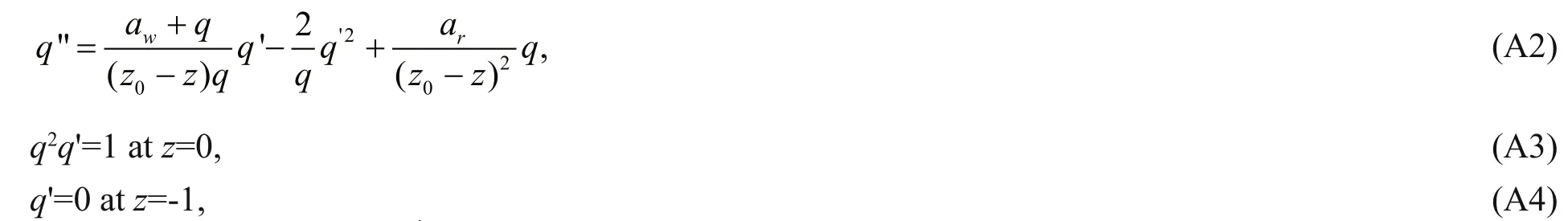
To solve above set of equations, we use the shooting method and consider the following system, in which for kthiteration q, as the function of the vertical coordinate z and an unknown boundary condition tksatis fies the following equation with Cauchy conditions at the base of the mixed layer z=-1,
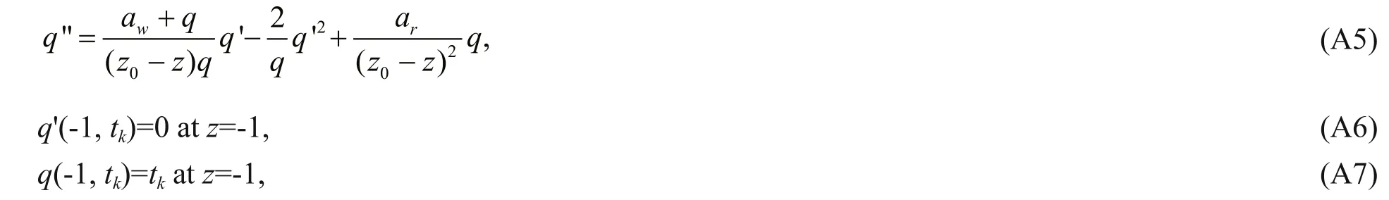
and an extra condition q2(0, tk) q'(0, tk)=1 at the surface z=0.
If the system is well converged, the following condition should be satis fied:

which leads to

and so

De fining two functions Y= ∂q/ ∂ t and Y'= ∂q'/ ∂ t, we have

Hence with an initial guess of the boundary value t1of the turbulent velocity at the base of the mixed layer,we solve respectively q and Y from following equations:


Then use Eq.A11 to get the value of t2, from which a new set of equations can be obtained. The cycle goes on tillis smaller than a prescribed small number.
2 Comparison of model results against observations
Black dots in Fig.3 denote dissipation rate calculated from dissipation-scale velocity fluctuations made with airfoil lift probes mounted on the Advanced Microstructure Pro filer (AMP) within a warm-core Gulf Stream ring during a cold-air outbreak (Shay and Gregg, 1984). These pro files were formed of seven bursts of drops taken during the cold air-break; each burst contained 4–12 pro files and was taken during an interval of between 1 and 3 h. The seven bursts spanned a period of 27 h when the mixed layer depth increased from 70 m to 170 m. Based on closeness of observed data for the atmospheric forcing including the work of surface wind stress and surface buoyancy flux, we obtain three sets of Ew, Jb0and H, and use each of them to estimate u*and w, which were subsequently used as input to our simple turbulence model. The three blue lines in Fig.3 are for the three sets with a=0.52, the three red lines are for a=1, and the three black lines are for w=0.
3 Global distribution of TKE dissipation rate and mixing coefficient
猜你喜欢
Chinese Physics B(2022年6期)2022-06-29
小天使·一年级语数英综合(2019年8期)2019-08-27
故事会(2019年10期)2019-05-27
人大建设(2018年12期)2018-03-21
电影文学(2017年10期)2017-12-27
作文·初中版(2017年10期)2017-10-25
作文·初中版(2017年8期)2017-09-04
作文·初中版(2017年8期)2017-09-04
作文·初中版(2017年2期)2017-03-06
 Journal of Oceanology and Limnology2018年4期
- Journal of Oceanology and Limnology的其它文章
- Editorial Statement
- Recent insights into physiological responses to nutrients by the cylindrospermopsin producing cyanobacterium,Cylindrospermopsis raciborskii*
- Response of Microcystis aeruginosa FACHB-905 to different nutrient ratios and changes in phosphorus chemistry*
- In fluence of light availability on the speci fic density, size and sinking loss of Anabaena flos- aquae and Scenedesmus obliquus*
- Application of first order rate kinetics to explain changes in bloom toxicity—the importance of understanding cell toxin quotas*
- Regime shift in Lake Dianchi (China) during the last 50 years*