
A Pressure Parametric Dark Energy Model∗
2018-12-13 06:33JunChaoWang王俊超andXinHeMeng孟新河
关键词:新河
Jun-Chao Wang(王俊超) and Xin-He Meng(孟新河)
Department of Physics,Nankai University,Tianjin 300071,China
AbstractIn this paper,we propose a new pressure parametric model of the total cosmos energy components in a spatially flat Friedmann-Robertson-Walker(FRW)universe and then reconstruct the model into quintessence and phantom scenarios,respectively.By constraining with the datasets of the type Ia supernova(SNe Ia),the baryon acoustic oscillation(BAO)and the observational Hubble parameter data(OHD),we find thatat the 1σ level and our universe slightly biases towards quintessence behavior.Then we use two diagnostics including Om(a)diagnostic and state finder to discriminate our model from the cosmology constant cold dark matter(ΛCDM)model.From Om(a)diagnostic,we find that our model has a relatively large deviation from the ΛCDM model at high redshifts and gradually approaches the ΛCDM model at low redshifts and in the future evolution,but they can be easily differentiated from each other at the 1σ level all along.By the state finder,we find that both of quintessence case and phantom case can be well distinguished from the ΛCDM model and will gradually deviate from each other.Finally,we discuss the fate of universe evolution(named the rip analysis)for the phantom case of our model and find that the universe will run into a little rip stage.
Key words:dark energy model,quintessence,phantom,Om diagnostic,state finder,the rip
1 Introduction
The conventional Einstein field equation dominated by matter without negative pressure(Gµν=8πGTµν)and Hubble law leads to the conclusion that the universe is in a decelerating expansion period.However,since the reported results of the accelerated expasnion of the universe from the supernova data observed in 1998[1]and 1999,[2]further observations consistently show that that the current universe is in the phase of accelerated expansion.In order to physically account for the phenomenon,one way is to modify the left side of the traditional Einstein field equation(modify the gravity).Another way is to add a negative pressure matter component named dark energy to the right side of the equation.One of the global fitting well scenarios is the so-called standard cosmology or the ΛCDM model,which includes the simplest dark energy model with the equation of state(EoS)ω ≡ p/ρ= −1 that provides a reasonably good account of the properties of the currently observed cosmos such as accelerating expansion of the universe,the large-scale structure and cosmic microwave background(CMB)radiation.However,there has a major problem(named the fine-tuning problem)that the observed value of dark energy density is 120 orders of magnitude smaller than the theoretical value in quantum field theory if taking the allowed highest energy cut o ffscale as the Planck mass;[3−4]besides,there is also the so called coincidence problem,which asks why dark energy density and physical material density are exactly in the same order of magnitude.To alleviate these problems,some extended models have been raised such as an evolving scalar field with the time variant EoS,for example.
In order to study the characterization of dark energy component,one of the feasible methods is to parameterize some observable physical quantities and then use the observed data to quantify the parameters.The mainstream is the EoS parametrization,such as Chevalier-Polarski-Linder(CPL)[5−6]parametrization ωde(z)= ω0+ωaz/(1+z)which behaves as ωde→ ω0for z → 0 and ωde→ ω0+ωafor z→ ∞.A few years later a more general form ωde(z)= ω0+ ωaz/(1+z)pnamed Jassal-Bagla-Padmanabhan(JBP)[7]parametrization has been proposed.In addition,Wetterich[8]has also given a parametric form which goes by ωde(z)= ω0/[1+bln(1+z)]2and it behaves as ωde→ ω0for z → 0 and ωde→ 0 for z→∞.
In recent years,some pressure parametric models for the mysterious dark energy or total energy components have been continuously proposed.In 2008,Sen,Kumar,and Nautiyal[9−10]have put forward a pressure parametric model of dark energy
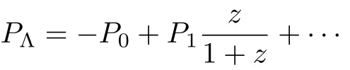
Seven years later,Zhang,et al.,[11−12]have proposed two dark energy models for the total pressure P(z)=Pa+Pbz and P(z)=Pc+Pd(z/(1+z)).Then,two years latter,Wang,Yan,and Meng[13]have raised a pressureparametrization unified dark fluid model P(z)=Pa+Pb(z+z/(1+z)).In the following of this paper we give out a new pressure parametric model of the total energy components as P(z)=Pa+Pbln(1+z),(z≠ −1)in a spatially flat FRW universe and then we discuss its property detailedly.
To investigate the model properties in details,this paper is organized as follows:In Sec.2,we propose the parametric model by continuously previous studying with the essential formalism and discuss the meanings for the two parameters of the model analytically.Section 3 is the reconstructions of our model with the quintessence and phantom scalar fields,respectively.In Sec.4,we constrain our model by using data from SNe Ia,BAO and OHD.In Sec.5,we discriminate our model from the ΛCDM model by using Om(a)diagnostic and the state finder parameters.Section 6 shows the discussions about the fate of universe evolution named the rip analysis for the phantom case of proposed model.In the last section,Sec.7,the conclusions and discussions are given.
2 The Parametric Model
Though two decades have passed a consistent and convincing dark energy theory is yet to come.To understand the puzzling dark energy physics better and by keeping on our exploration,we can properly parameterize its pressure.For example,one can hypothesize a relation between the pressure and the redshift,then integrate out the expression of the density ρ through the conservation equation.Finally from the Fridemann equations H2=(8πG/3)∑iρiand the EoS ω =P/ρ we are able to get the form of the Hubble parameter H and ω expression,respectively.By this treatment so far,a closed system for the evolution of the universe has been established,which is described by the Friedmann equations,the conservation or continous equation and the EoS form.
Assume a relationship between the pressure of all energy components in the universe and the redshift as below,

where Paand Pbare free parameters.We make this assumption because the form of ln(1+z)=z−(z2/2)+(z3/3)− ···for|z|<1 and it may be much helpful for providing more opportunities to further other studies related.When Pb=0,the model is reduced to the well known ΛCDM model;while when Pb≠0,the total pressure gives more interesting properties.By using the relation of scale factor a=1/(1+z)and the conservation equation,we have
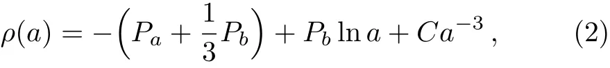
where C is an integration constant.We assume that ρ0is the present-day energy density i.e.ρ(a=1)= ρ0.Finally the total energy density and pressure can be integrated separately as
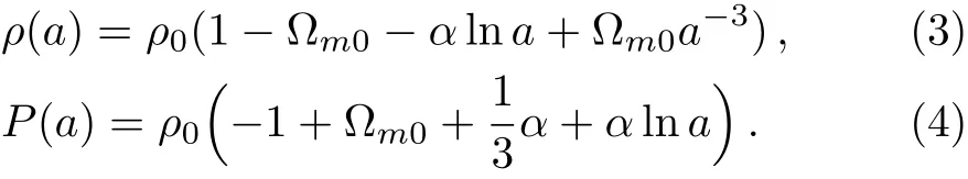
Here the parameters(Pa,Pb)are replaced by new dimensionless parameters(α,Ωm0)where α ≡ −Pb/ρ0andΩm0≡ (1/ρ0)(ρ0+Pa+(1/3)Pb).
In this model,ρ(a)contains cosmic matter contribution Ωm0a3and the cosmic dark energy composition 1−Ωm0−αlna.If we require that the density of each component would be greater than zero,then ρde/ρ0=1−Ωm0+αln(1/a)>0,so the part of a>exp((1−Ωm0)/α)>1 if α >0 and a
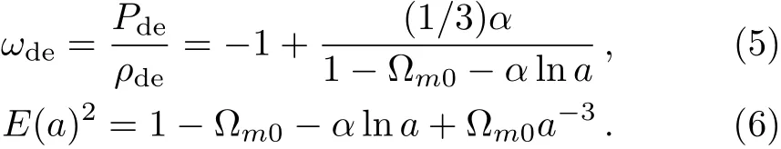
To exhibit dark energy better,we derive the density ratio parameter of the dark energy as follows
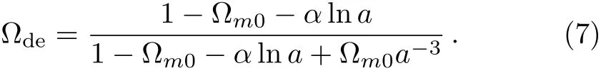
Two parameters α and Ωm0will be constrained by observations in the following section.On the one hand,when a=1,Ωm=1−Ωde= Ωm0.So Ωm0is the presentday matter density parameter.On the other hand,when α =0,the model reduces to the flat ΛCDM model.Further,we can see clearly that in the next section,the α>0 for the quintessence case while α<0 corresponded to the phantom case.
3 The Reconstructions
Unlike the ΛCDM model,this scenario gets the dynamical dark energy within.The natural way to introduce varying dark energy is to assume a scalar field that changes over time and the corresponding pressure and energy are respective i.e.Pde=Pscalar,ρde= ρscalar.In this section,we discuss the quintessence and phantom scalar field separately.Consider the dark energy as a real scalar field ϕ with the action of stress energy,which can be written as
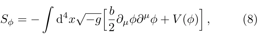
where(b/2)gµν∂µϕ∂νϕ is the kinetic energy and V(ϕ)is the potential energy,b=1 or−1 corresponding to the quintessence case and phantom case,respectively.And the stress-energy tensor is
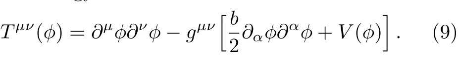
If we regard the scalar field as a perfect fluid,the energy density and pressure of the scalar field can be written as
Assume ϕ is uniform in space and only relies on time i.e.ϕ= ϕ(t),then Eqs.(10)and(11)can be simplified to
where the dot denotes the derivatives w.r.t.the cosmic time.
3.1 The Quintessence Case
Assume the universe consists of quintessence and matter.By comparing Eqs.(3)and(4)with Eqs.(12)and(13),we can obtain
Simplify the above two equations,then we have
where Mpl≡ (8πG)−1/2and.In Eq.(18),“±” corresponds to two solutions.Only when α >0,Eq.(18)is meaningful.So α>0 corresponds to the quintessence case.And from Eq.(5)we know that at this time ωde> −1.
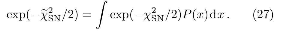
From Eqs.(17)and(18)we can draw the relation between ϕ(a)and V(ϕ)shown in Fig.1.In Fig.1,from the upper panels we know that ϕ increases as a increases while V decreases as ϕ increases.The lower panels show that ϕ decreases as a increases while V decreases as ϕ decreases.So for quintessence case,V decreases as a increases and it implies ρdewill decrease in the future.
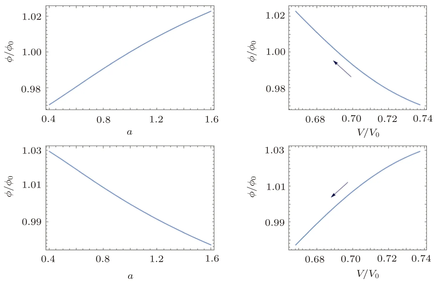
Fig.1 The quintessence field ϕ/ϕ0versus the scale factor a,and the quintessence field ϕ/ϕ0versus the potential V/V0(assume ϕ0= ϕ(a=0)=1 and V0= ρ0).The upper and lower panels correspond to the plus and minus sign in Eq.(18),respectively.The arrows indicate the evolutional directions of the potential,and we have used Ωm0=0.3 and α =0.05 numerically.
3.2 The Phantom Case
Assume the universe consists of phantom and matter.By comparing Eqs.(3)and(4)with Eqs.(12)and(13),we can obtain
Subsequently,by solving the above two equations,one can derive
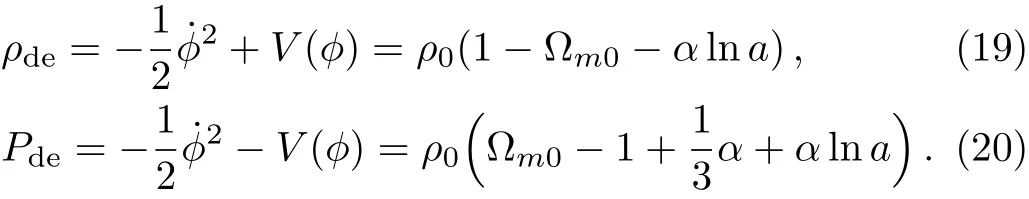
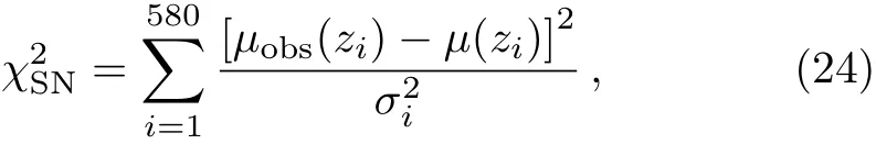
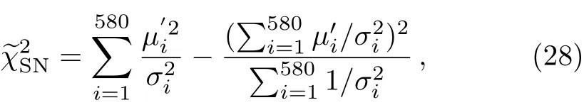
From Eqs.(22)and(23)we can draw the relation between ϕ(a)and V(ϕ)shown in Fig.2.In Fig.2,from the upper panels we know that ϕ increases as a increases while V increases as ϕ increases.And the lower panels show that ϕ decreases as a increases while V increases as ϕ decreases.So for the phantom case,V increases as a increases,which implies ρdewill increase in the future and lead H→∞as a→∞,and universe will get rip in the end.
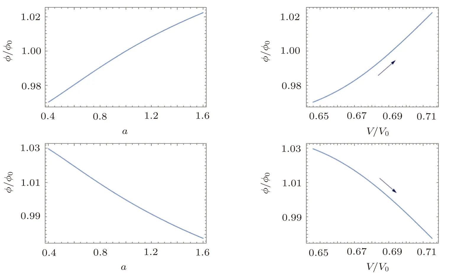
Fig.2 The phantom field ϕ/ϕ0versus the scale factor a,and the phantom field ϕ/ϕ0versus the potential V/V0(assume ϕ0= ϕ(a=0)=1 and V0= ρ0).The upper and lower panels correspond to the plus and minus sign in Eq.(23),respectively.The arrows indicate the evolutional directions of the potential.We have used Ωm0=0.3 and α = −0.05 numerically.
4 The Constraints
4.1 Type Ia Supernova
Measuring the distance by the light curve of a supernova is one of the most accurate ways to measure the distance to the universe.In this paper we use the Union2.1 SNe Ia dataset,[14]which contains 580 SNe Ia.First,we minimize the chi-square
whereµobs(zi)is the observed distance modulus,σiis the 1σ level of the observed distance modulus for each supernova andµ(zi)is the theoretical distance modulus which is defined as
where H0is the Hubble parameter at z=0,C is the zero value of the distance modulus and DLis the Hubblefree luminosity distance in a spatially flat FRW universe,which can be written as
where E(z)is the dimensionless Hubble parameter.Since the zero value C in Eq.(25)of the distance modulus measured in the astronomical observation is arbitrarily selected,H0is also arbitrary.In Eq.(25),H0appears in 5lnH0.Assume x=5lnH0for a uniform distribution,P(x)=1.Then the likelihood for marginalize x can be written as
By solving Eq.(27),we get the marginalized result
4.2 Baryon Acoustic Oscillations
BAO is the fluctuations of the visible baryonic matter density on the length scale after the pre-recombination universe,and the BAO peak is centered on a comoving distance equal to the sound horizon at the drag epoch,rs.BAO can be measured in the transverse and radial direction.The transverse measurement DLH0/(1+z)rsis sensitive to the photometric redshift,where DLis the Hubble-free luminosity distance shown in Eq.(26);While the radial measurement DH/rsis correlative to the Hubble parameter H(z),where DH=c/H0E(z)is the Hubble distance.The geometrical mean of radial and transverse distance named the volume averaged comoving angular diameter distance Dv(z)is given by
Then we get the observables d(z)and A(z)which can be written as
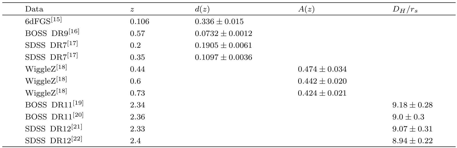
Table 1 The BAO data at the 1σ level used in this paper.
In this section,H0and rsare the extra parameters so we use the data of Plank15 for H0=67.3 km ·s−1·Mpc−1and rs=147.33 Mpc.And the BAO data used in this paper are listed in Table 1.Next,by using the datasets Refs.[15–22],we need to calculate the chi-squares respectively,which are written as
and
And then we get

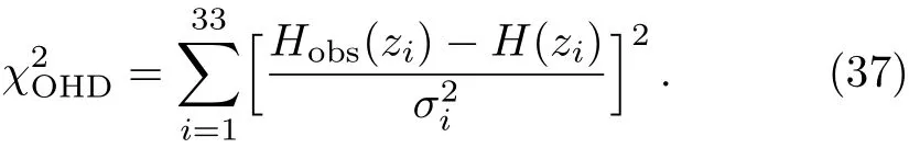
4.3 Observational Hubble Parameter Data
The observational methods for H0are the differential age method,the radial BAO size method and the gravitational wave method.In this paper,we use a compilation of 33 uncorrelated data points measured by the differential age method listed in Table 2.
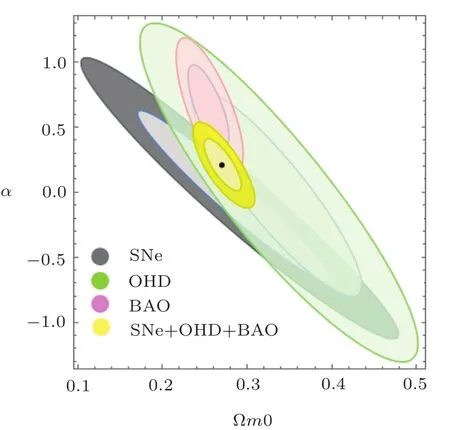
Fig.3 (Color online)The 1σ and 2σ level ranges of the model parameter pair(Ωm0,α)for using SNe Ia data(grey),OHD data(green),BAO data(pink)and the combined data of SNe Ia+OHD+BAO(yellow).
Then we need to figure out

The observational constraints on the model parameter pair(Ωm0,α)are shown in Fig.3;The best- fit values at the 1σ level of parameters Ωm0and α from the joint constraints SNe Ia+BAO+OHD are listed in Table 3;The relations of(a,ωde),(a,q)and(a,Ωde)compared with our model for the best- fit values,which is the quintessence case and the ΛCDM model for Ωm0=0.27 are shown in Fig.4,where q(a)is the deceleration parameter written as
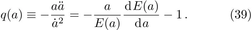
Table 2 The observational Hubble parameter data measured by the differential age method used in this paper.
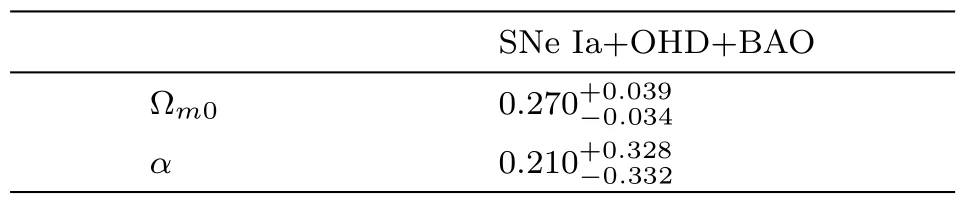
Table 3 The best- fit values at the 1σ level of parameters Ωm0and α from the joint constraints SNe Ia+BAO+OHD.
From Fig.3 and Table 3,we can see that the range of Ωm0is acceptable and the range of α supports quintessence behavior slightly.But it can not be completely excluded phantom case at the 1σ level. From Fig.4,the evolutionary trajectories of ωde,q and Ωdecan’t be distinguished from the ΛCDM model at the 1σ level.Therefore,we will adopt the Om diagnostic and state finder to discriminate our model from the ΛCDM model better.From Fig.4(b),we can find that the universe of our model is accelerating expansion,which fits the observation.Interestingly,from Fig.4(c),it seems thatΩdeof our model will gradually coincide with the ΛCDM one,which tends to be a de Sitter universe.But in this model,for the quintessence case(the shaded region above the red dashed line in Fig.4(c)),if we extend a,we can find Ωdestarts to go down,which is very different from the ΛCDM model.
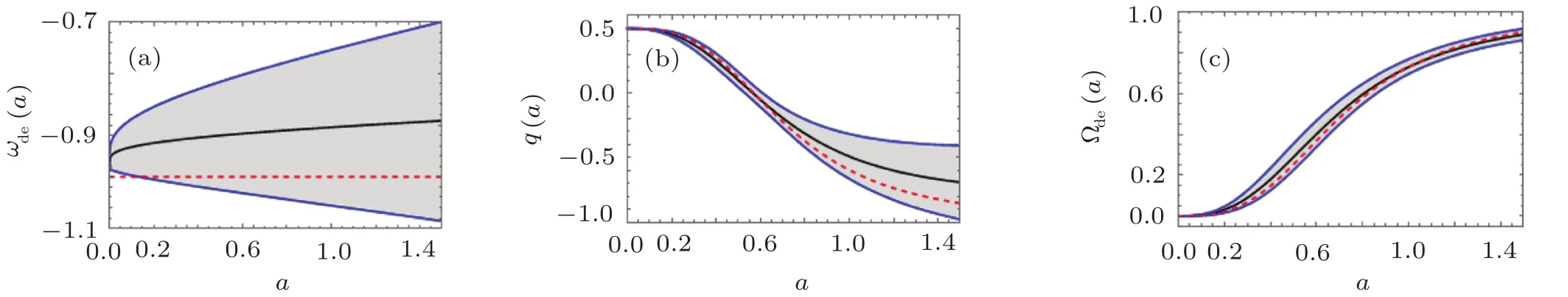
Fig.4(Color online)The relations of(a,ωde)(a),(a,q)(b),and(a,Ωde)(c)compared with our model and the ΛCDM model.The black line and red dashed line correspond to our model with the best- fit values listed in Table 3 and the ΛCDM model with Ωm0=0.27,respectively.The shaded region and blue lines represent the 1σ level regions and corresponding boundaries.
For the phantom case(the shaded region below the red dashed line in Fig.4(c)),although Ωdeof our model rises monotonously as same as the ΛCDM model,it will go to a little rip in the final while the ΛCDM model will go to the pseudo-rip.The detail of rip will be discussed at the rip section below.
5 Discriminations byOm(a)Diagnostic and the State finder
As more and more dark energy models are proposed so far,how to discriminate different dark energy models becomes an important and meaningful issue.In the first part of this section,we employ Om(a)diagnostic to distinguish our model with the best- fit values from the ΛCDM model.In the second part,we use the state finder parameters to discriminate among the quintessence picture,the phantom picture and the ΛCDM model.
5.1 Om(a)Diagnostic
The Om(a)diagnostic[31]is a geometrical method,which combines Hubble parameter and redshift to discriminate the dark energy models by measuring their deviation from the ΛCDM model.Om is defined as
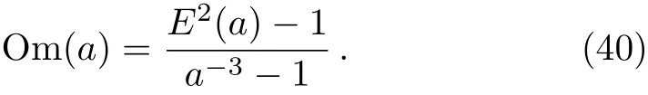
For a spatially flat ΛCDM model,E2(a)= Ωm0a−3+(1−Ωm0).So Om(a)|ΛCDM− Ωm0=0,which provides a null test of ΛCDM hypothesis.
In Fig.5,we plot the evolutionary trajectories of our model and the ΛCDM model.From Fig.5,we can see that our model has a relatively large deviation from the ΛCDM model at high redshifts and gradually approaches the ΛCDM model at low redshifts and in the future evolution.But they can be easily distinguished from each other at the 1σ level all along.The Om diagnostic discriminates our model from the ΛCDM model very well.
Fig.5(Color online)The Om diagnostic for our model and the ΛCDM model.The black line represents our model with the best- fit values listed in Table 3.The red dashed line represents the ΛCDM model with Ωm0=0.3.The shaded region and blue lines represent the 1σ level regions and corresponding boundaries.
5.2 State finder
The Om(a)diagnostic relies on the first order derivative of the scale factor with the respect to cosmic time alone while the state finder[32]relies on the higher order derivatives.The geometric parameter pair(r,s)are deif ned as
where q is the deceleration parameter shown in Eq.(39).By using Eqs.(41)and(42)we can derive q and s of our model and the ΛCDM model,and they are listed in Table 4.For the better comparison,we also list the dimensionless Hubble parameter E,the density ratio parameter of the matter Ωmand the deceleration parameter q in Table 4.
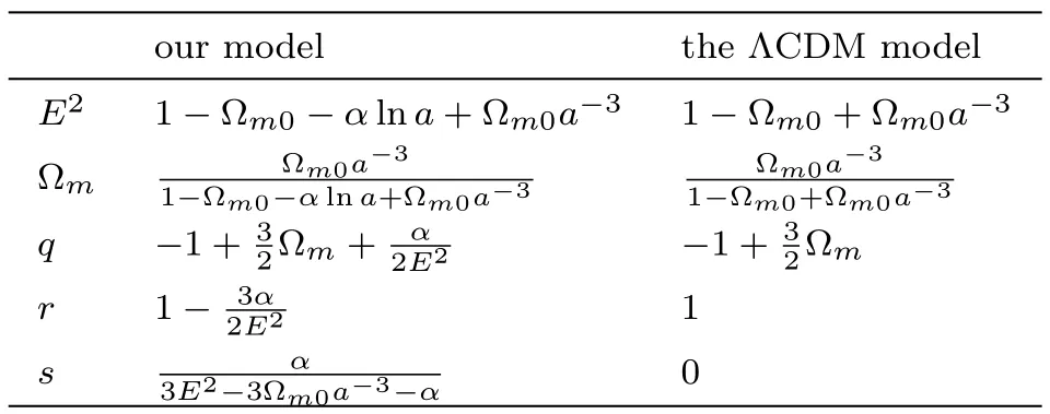
Table 4 The comparison of different parameters between our model and the ΛCDM model.
Figure 6 shows the relation between q and r.The relation between r and s is shown in Fig.7.Both of two if gures indicate that the quintessence case and the phantom case can be well distinguished from the ΛCDM model and will gradually deviate from each other.Interestingly,in Fig.7,when two cases deviate slightly from a=0,they both oscillate up and down at point(1,0)and constantly overlap.Then they quickly move away from point(1,0)in the opposite directions and immediately tend to be stabilized and part ways.It implies that this two cases may share the same phase at the birth of the universe.
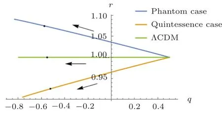
Fig.6 (Color online)The state finder pair(q,r)for quintessence case(blue line),phantom case(orange line)and the ΛCDM model(green line).Arrows represent the directions of time evolution.The spots indicate the present epoch.We have used Ωm0=0.3,α =0.05 for quintessence case,Ωm0=0.3,α = −0.05 for phantom case and Ωm0=0.3,α =0 for the ΛCDM model.
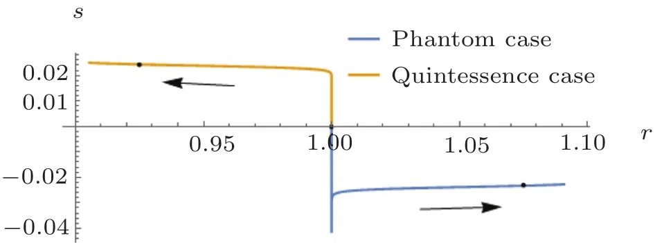
Fig.7 (Color online)The state finder pair(r,s)for quintessence case(blue line),phantom case(orange line)and the ΛCDM model(the fixed point(1,0)).Arrows represent the directions of time evolution.The spots indicate the present epoch.We have used Ωm0=0.3,α =0.05 for quintessence case and Ωm0=0.3,α = −0.05 for phantom case.
6 The Rip
From the conservation equation˙ρ=−3Hρ(1+ω)we know that the density will increase in the future when the EoS of dark energy ωde< −1 which corresponds the phantom case.Based on various evolutionary behaviors of H(t),we divide the ultimate fates of the universe into the following categories:[33](i)The big rip,for which H(t)→∞at finite time.At that time,the dark energy density is in finity and produces an in finite repulsion,the gravitationally bound system will be dissociated in order of large to small.[34](ii)The little rip,for which H(t)→∞at in finite time.This scenario has no singularity in the future whereas also leads to a dissolution of bounds tructures at some point in the future.[35](iii)The pseudo-rip,for which H(t)→constant,which is an intermediate case between the de Sitter cosmology and the little rip.Next,we will make a rip analysis for the phantom case of our model briefly.For our model,the Hubble parameter is

When a→∞,Eq.(43)can be simplified as
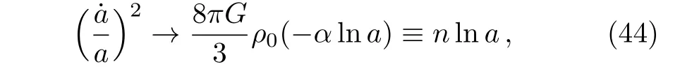
where n ≡ −(8πG/3)ρ0α. By solving the differential Eq.(44),we can obtain the scale factor a as a function of time t

where t0is the present value of time.Substitute Eq.(45)to Eq.(44),we get
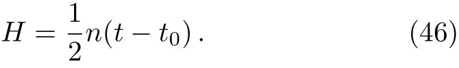
From Eq.(46)we can find H(t)→∞as time goes to in finity.So the ultimate fate of the phantom case of our model is the little rip.
7 Conclusions and Discussions
In this paper,we propose a pressure parametric model of the total energy components in a spatially flat FRW universe.This model has two parameters Ωm0and α where Ωm0is the present-day matter density parameter and α displays the model difference from the flat ΛCDM model. By constraining with the datasets of SNe Ia,BAO and OHD,we find that Ωm0=and α=at the 1σ level indicating that our universe slightly biases towards quintessence behavior while it can not be completely excluded phantom at the 1σ level.It also implies that our model includes the ΛCDM model when α=0.Then we use Om(a)diagnostic to discriminate our model with the best- fit values from the ΛCDM model.We find that our model deviates relatively far from the ΛCDM model at high redshifts and gradually approaches the ΛCDM model in the future.However they can be easily distinguished from each other at the 1σ level all along.Next,we use the state finder to discriminate among the quintessence case,the phantom case and the ΛCDM model.Both of panels(q,r)and(r,s)indicate that quintessence and phantom scenarios can be well distinguished from the ΛCDM model and will gradually deviate from each other.Finally,we discuss the fate of universe evolution named the rip analysis for the phantom case of our model and find that the universe will run into a little rip stage,which has no singularity in the future whereas also leads to a dissolution of bound structures at some point in the future.
On the one hand,dark energy phenomenon has appeared about two decades,but we still do not know its physical reality.While waiting for upcoming new observations,lots of theoretical efforts need continuously paid with the hope we can understand it better.On the other hand,the constraints give a tiny α,so this model can also provide a possible solution for other studies to approximate the pressure at low redshifts.
猜你喜欢
结构工程师(2022年2期)2022-07-15
今日农业(2021年10期)2021-11-27
江苏教育·书法教育(2020年5期)2020-09-10
江苏教育·书法教育(2020年5期)2020-09-10
江苏教育·书法教育(2020年5期)2020-09-10
今日农业(2019年11期)2019-08-15
读书文摘·经典(2018年1期)2018-01-10
岷峨诗稿(2014年1期)2014-11-15
治淮(2013年3期)2013-03-11
 Communications in Theoretical Physics2018年12期
- Communications in Theoretical Physics的其它文章
- Mixed Local-Nonlocal Vector Schrödinger Equations and Their Breather Solutions∗
- Circular Semi-Quantum Secret Sharing Using Single Particles∗
- Existence and Dynamics of Bounded Traveling Wave Solutions to Getmanou Equation∗
- Runaway Directions in O’Raifeartaigh Models∗
- The 1/NcExpansion in Hadron Effective Field Theory∗
- Quasinormal Modes of the Planar Black Holes of a Particular Lovelock Theory∗