
A Renormalized-Hamiltonian-Flow Approach to Eigenenergies and Eigenfunctions∗
2019-07-25 02:01WenGeWang王文阁
关键词:文阁
Wen-Ge Wang (王文阁)
Department of Modern Physics,University of Science and Technology of China,Hefei 230026,China
Abstract We introduce a decimation scheme of constructing renormalized Hamiltonian flows,which is useful in the study of properties of energy eigenfunctions,such as localization,as well as in approximate calculation of eigenenergies.The method is based on a generalized Brillouin-Wigner perturbation theory.Each flow is specific for a given energy and,at each step of the flow,a finite subspace of the Hilbert space is decimated in order to obtain a renormalized Hamiltonian for the next step.Eigenenergies of the original Hamiltonian appear as unstable fixed points of renormalized flows.Numerical illustration of the method is given in the Wigner-band random-matrix model.
Key words: generalized Brillouin-Wigner perturbation theory,Hamiltonian flow,eigenfunction structure,eigenvalue
1 Introduction
Properties of energy eigenvalues and eigenfunctions are of central importance in a variety of fields,from nuclei physics,atomic physics,to condensed matter physics,and so on.[1−12]In particular,they are of relevance to thermalization,[13−21]a topic which has attracted renewed interest in recent years.An important method of studying these properties is the renormalization group method.Various versions of this method have been developed.For example,in calculating energy eigenfunctions in the low energy region,wide use has been made of Wilson’s numerical renormalization group[22−23]and of the density-matrix renormalization group method.[24−25]
Localization of wavefunctions is one of the most important phenomena discovered in the field of condensed matter physics[26−30]and in the field of quantum chaos.[31−32]A real-space renormalization-group method and its modified versions[33−38]have been found quite successful in the study of localization properties in one-dimensional systems with (effectively) finite range of coupling; while in the case of two and more than two-dimensional systems,they have been found successful only in some special cases such as the Fibonacci quasi-lattices (see,e.g.,Refs.[39–40]).Moreover,recently,the phenomenon of many-body location has attracted wide attention (see,e.g.,Refs.[41–44]).
Different schemes of constructing renormalized Hamiltonian flows are usually suitable for different types of problems.No scheme has been found universally useful.Hence,it is always of interest to find new schemes of constructing renormalized Hamiltonian flows.
In this paper we introduce a new method of constructing renormalized Hamiltonian flow,based on a generalized Brillouin-Wigner perturbation theory (GBWPT).[45−49]The GBWPT shows that an arbitrary eigenfunction of a Hamiltonian can be divided into two parts,a perturbative part and a non-perturbative part,with the perturbative part expanded in a convergent perturbation expansion in terms of the non-perturbative part.Making use of this result of the GBWPT,we show that a subspace of the Hilbert space,which is associated with a perturbative part of the eigenfunction,can be decimated.This decimation scheme produces a renormalized Hamiltonian and,following this procedure,a renormalized Hamiltonian flow can be constructed.
We show that,for a renormalized Hamiltonian flow constructed by the method mentioned above,eigenenergies of the original Hamiltonian appear as(unstable)fixed points of a property of the flow.Furthermore,those eigenfunctions of the renormalized Hamiltonians in the flow,which share the same eigenenergy,have related components.These two properties of the renormalized Hamiltonian flow may be made use of in approximate calculation of eigenenergies and in the study of properties of the eigenfunctions of the original Hamiltonian,e.g.,their localization properties.These predictions are checked numerically in the Wigner-band random-matrix model.
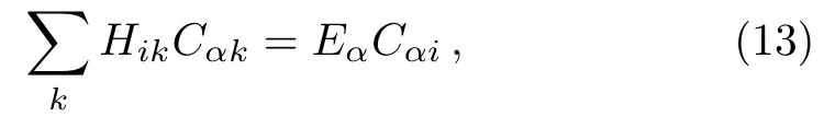
2 General Theory
2.1 Generalized Brillouin-Wigner Perturbation Theory
In this section,we discuss the basic contents of GBWPT.It is a direct generalization of the ordinary Brillouin-Wigner perturbation theory,which can be found in textbooks,e.g.,in Ref.[50].Consider a perturbed HamiltonianH=H0+V,whereH0is an unperturbed Hamiltonian andVis a generic perturbation.In the normalized eigenbasis ofH0,denoted by
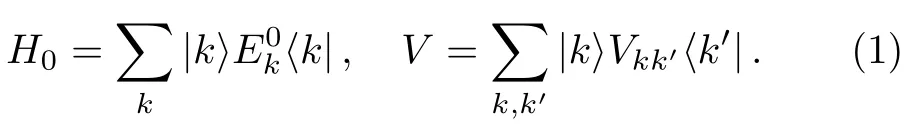
For an energy eigenstate|α〉,let us divide the setinto two subsets,denoted bySαand,respectively.This gives two projection operatorsPandQ,
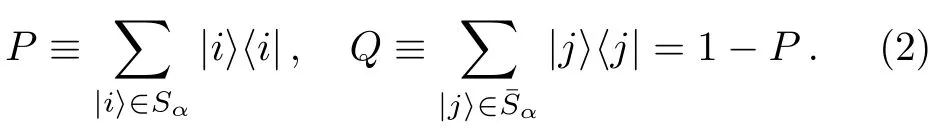
Here we useto indicate basis statesinSαandforCorrespondingly,the stateis divided into two parts,


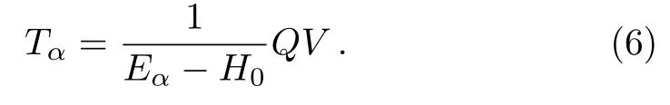
Multiplying both sides of Eq.(4) byQand noticing thatQH0=H0Q,one has

where
Substituting Eq.(5) into Eq.(3) and doing iteration,one finds thatcan be expanded in a convergent perturbation expansion,
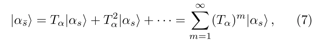
when the following condition is satisfied
When the setSαincludes only one basis vector,the expansion in Eq.(7) gives the ordinary Brillouin-Wigner perturbation expansion.Since the exact eigenenergyEαappears in the expansion,the expansion can not be immediately employed in numerical computation.However,noticing thathas one component only in the basisand that the componentsCαkshould satisfy certain normalization condition,this problem can be overcome.For example,taking the normalization condition=1 for normalizedand multiplying Eq.(4) from left byone can write the exact energy asEα=E0i+Then,one can writeEαandin the form of two related iterative expansions.[50]
In the case thatSαincludes more than one vectorsEq.(7) gives a generalization of the (ordinary) Brillouin-Wigner perturbation theory(GBWPT).In this case,since there are at least two componentsCαiin,merely making use of the normalization condition,one can not writeEαandin two related iterative expansions.Therefore,in the GBWPT,Eαandcan not be calculated in a way similar to that discussed above in the ordinary Brillouin-Winger perturbation theory.
Several applications of the GBWPT have been found.The condition (8) determines the separation ofinto two parts,and.In systems with band structure of the Hamiltonian,usuallycorresponds to the main body of,whilecorresponds to the tail part ofwith small components.[45,48]It has been shown that the expansion in Eq.(7) is useful in deriving analytical expressions for the decaying behavior of the tails of[45,48]This separation ofhas also been found useful in approximate calculation of eigenstates in certain energy region.[47]Further numerical investigation reveals that this separation of energy eigenstates is useful in the study of phenomenon like dynamical localization[46,48]and in the study of the distribution of components of wave functions in quantum chaotic systems.[49]
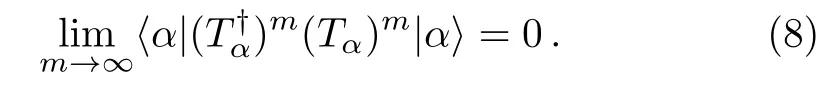
In this paper,we discuss a new application of the GBWPT,namely,a general scheme of constructing renormalized Hamiltonian flow.Before doing this,it is useful to give further discussion for the condition of separating an energy eigenstate into the two parts discussed above.A sufficient (unnecessary) condition for Eq.(8) to hold is

In order to understand better the condition (9),we insert the expression of the projection operatorQgiven in Eq.(2) into Eq.(6) and get
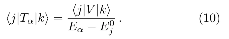
It is seen that only basis statesgive contribution to the denominator ofTα.Therefore,as long as the setis chosen such that allE0jofare far enough fromEα,Eq.(9) and hence Eq.(7) hold.This gives a convenient way of doing the separation of
An advantage of using Eq.(9)is that one does not need to know the exact statein advance.Equation (9) is also useful when we treat a HamiltonianHwith a degenerate spectrum.As well known,degenerate spectrum ofHmay bring problem to the ordinary perturbation theory.However,in the GBWPT,Eq.(7)can still hold whenHhas a degenerate spectrum.In fact,since Eq.(9) does not contain any eigenstate,for eigenstates with the same eigenenergyEα,this equation gives the same separation of the basis states,i.e.,the setSα.For such a separation,Eq.(7) holds for all the eigenstates with the eigenenergyEα.In this case,Sαincludes more than one basis vectors.Different eigenstateswith the same eigenvalueEαhave different componentsCαiin,hence,have differentdetermined by Eq.(7).
For the above reasons,in what follows,we use Eq.(9)to determine the separation ofinto the two partsand
2.2 Renormalized Hamiltonian
A renormalized Hamiltonian can be constructed for an eigenstateofH,by decimation of the statesinFor this purpose,making use of Eq.(7),we writeas
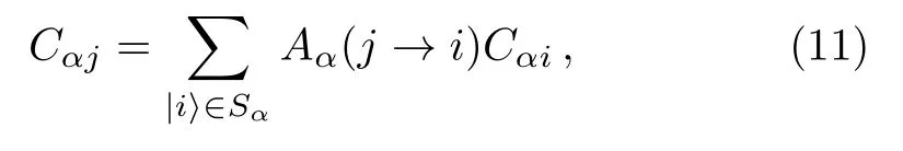
where
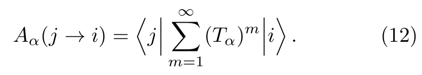
replacingCαjby the right hand side of Eq.(11),one has
where
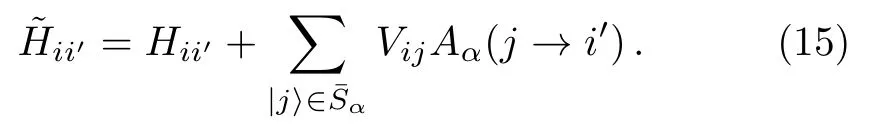
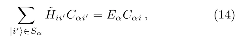
This suggests that a renormalized Hamiltoniancan be introduced,
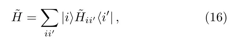
which is an operator in the subspace spanned by states∈Sα.The most important relation betweenHandis that the stateis an eigenstate ofwith the eigenenergyEα,as shown in Eq.(14).Note that the elementsare functions ofEα.
WhenHhas a degenerate spectrum,as discussed in the previous section,degenerate eigenstates with the same eigenenergyEαshare the same separationSα,hence,they have the same quantitiesAα(j →i′).As a result,degenerate eigenstatesare eigenstates of the same renormalized HamiltonianTherefore,the above scheme also works in the case of degenerate spectrum.
The structure of non-zero off-diagonal elements ofHin the basisis usually different from that ofin.Indeed,Eqs.(12)and(15)show thatis typically nonzero when eitherHii′≠0 or there is a path of coupling fromtothrough statesin the set.Therefore,the number of basis stateswhich are coupled tobyis equal to or larger than that byH.
We remark that the condition (8),which guarantees the expansion in Eq.(7),can not completely fix the setSα.Hence,one usually has much free space in choosingSαin constructing a renormalized Hamiltonian.
2.3 Renormalized Hamiltonian Flow
Repeating the procedure discussed in the previous section,withplaying the role ofH,one can obtain a new renormalized Hamiltonian from ˜H.Following this,a renormalized Hamiltonian flow can be constructed,which is specific for the eigenstatewith eigenenergyEαof the original HamiltonianH.However,this method of constructing Hamiltonian flow has a drawback,namely,andEαare usually unknown.(The purpose of constructing a renormalized Hamiltonian flow is usually just to study properties ofandEα.) To avoid this drawback,in what follows we propose a more general method of constructing renormalized Hamiltonian flow,which is not specific for any eigensolution ofH.
Let us denote byH(0)the original HamiltonianH,byEα(0)andits eigenenergies and eigenstates,respectively.For a set of basis states in the Hilbert space ofH(0),denoted by{|k(0)〉},H(0)is divided into two parts as in Eq.(1),The set of basis states is also divided into two partsS(0)and,with∈S(0)and∈; correspondingly,two projection operatorsP(0)andQ(0)can be introduced in the same way as in Eq.(1).The components ofare denoted by
In considering the condition for a division of{|k(0)〉},let us write Eq.(9) in the following form,

where
HereEis a parameter with energy dimension,which is used in the construction of the renormalized Hamiltonian flow.Note that Eq.(17) gives Eq.(9) forE=Eα.
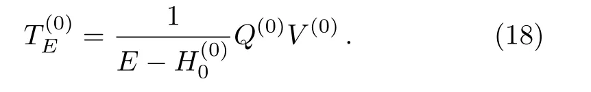
Then,we can decimate the basis states inand,similar toin Eq.(16),introduce the first renormalized Hamiltonianin the flow,
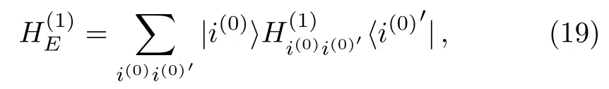
where

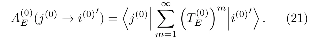
Here
ForE=Eα(0),similar to Eq.(14),we have

hence,Eα(0)is an eigenenergy ofH(1)EwithE=Eα(0).IfEis not equal to any ofEα(0),it is usually not an eigenenergy of.Note thatis an operator in the Hilbert space spanned by(0).
In the above procedure,with the superscript (0) replaced by Eq.(1),the second renormalized Hamiltonianin the flow can be constructed for the same parameterE.Then,with the superscript(1)replaced by Eq.(2),and so on,a renormalized Hamiltonian flowcan be constructed,withn=1,2,...
IfE=Eα(0)for a Hamiltonian flow thus obtained,an equation similar to Eq.(22)holds with 0 replaced byn−1 and 1 byn.This implies the following important relation betweenandH(0),that is,an eigenstateofhas the following relation to|α(0)〉,

whereis the same basis state asbut in the original labelling.This equation shows that some information in properties ofmay be obtained from properties of the corresponding eigenstateofIn the general case withEnot necessarily equal to any ofEα(0),let us denote byE(n)the closest eigenenergy oftoE.(Forn=0,takeH(0)).With increasingn,E(n)form a sequence with the flow,(E(0),E(1),E(2),...).IfE=Eα(0),Eq.(23) shows thatE(n)=Eα(0)for all values ofn; on the other hand,ifE≠Eα(0),E(n)are usually not equal toEα(0).Hence,Eα(0)are fixed points of the sequenceE(n),under the choice ofE=Eα(0).One may also consider the sequence of the deviation|Eα(n)−E|,for which zero is the fixed point corresponding to the choiceE=Eα(0).
2.4 An Efficient Method of Constructing Renormalized Hamiltonian Flow
The condition(17)with 0 replaced bynmust be satisfied,in order to constructfromHE(n)by decimating basis statesin.For a given choice of,it is usually not easy to prove whether the condition is satisfied or not.In fact,for an arbitrarily chosen setand an arbitrary value ofE,the condition is usually not satisfied.Therefore,it would be useful,if a general method can be found for decimation of an arbitrarily chosen set.In what follows,we introduce such a method.For brevity,in the following part of this section,we omit the superscript“(n)”,i.e.,all quantities should have the superscript“(n)”,except for the parameterE.
The technique is to first carry out a rotation in the subspace spanned by states∈,such thatHis diagonalized in the subspace.We assume that the number of states inis not large and it is not difficult to diagonalize numerically the sub-matrix of the HamiltonianHin this subspace.Let us denote bythe obtained eigenstates of the sub-matrix ofHin the subspace and byEjathe corresponding eigenenergies.
Now take the set ofas a new subset.Correspondingly,the HamiltonianHis divided into two parts,H0andV,in the same way as discussed in previous sections.In particular,by definition,is an eigenstate of,

Then,making use of the expression ofQin Eq.(2),we can writeTEin Eq.(18) as (with the superscript (0) replaced by (n) and then omitted)

whenEis not equal to any ofEja.Equation (25) implies that (TE)2=0,since there is no coupling among,namely,=0.As a result,Eq.(17) holds with 0 replaced byn.When it happens thatEis equal to one ofEja,one may change a little the two original subsetsSofandofby exchanging a few states in them; this may change the values ofEjaand makeE≠Eja.
Finally,by the method discussed in the previous section,the set of(equivalently,that of) can be decimated and a renormalized Hamiltonian can be obtained.In particular,AE(ja→i) has a quite simple expression,
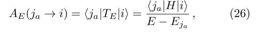
since (TE)2=0 for the choice of the set of.It is not difficult to see that the above schemes can work for a degenerate spectrum,as well.
3 Some Applications
In this section,we show that the method presented in this paper supplies a useful approach to properties of energy eigenvalues and eigenfunctions.
3.1 Eigenenergies as Unstable Fixed Points
As discussed in Subsec.2.3,the eigenenergiesEα(0)of the original HamiltonianH(0)are fixed points of the sequenceE(n),whereE(n)is the eigenenergy ofwhich is the closest toE.As a result of this property,the difference|E −E(n)|as a function ofE(withnfixed)has local minima at the positionsE=Eα(0).Hence,the eigenenergiesEα(0)can be calculated by finding out the local minima.In fact,numerical evaluation of eigenenergies of large-scale Hamiltonian matrices is a very important topic in many fields in physics.Various methods have been developed in dealing with this problem (see,e.g.,Refs.[47,51–57]).The renormalization group method discussed above supplies an alternative approach to this important problem.
To test the above predictions,we consider a banded random matrix model.Banded random matrix models have applications in several fields and are still under investigation (see,e.g.,Refs.[58–62]).Here we consider the so-called Wigner Band Random Matrix (WBRM) model,which was first introduced by Wigner more than 50 years ago for the description of complex quantum systems as nuclei.[63]It is still of interest (see,e.g.,Refs.[46,48,64–70]),since it is believed to provide an adequate description also for some other complex systems,e.g.,the Ce atom[71]and as well as dynamical conservative systems possessing chaotic classical limits.
We consider the following form of the Hamiltonian matrix in the WBRM model,

whereE0k=k(k=1,...,N),off-diagonal matrix elementsvkk′=vk′kare random numbers with Gaussian distribution forand are zero otherwise,andλis a running parameter for adjusting the perturbation strength.Herebis the band width of the Hamiltonian matrix andNis its dimension.
The theory discussed above predicts that the pointsE=Eα(0)are fixed points for the propertyE(n)of the renormalized Hamiltonian flow.To check this numerically,we consider original HamiltoniansH(0)as given in Eq.(27),whose dimensions are not very large such that they can be diagonalized directly by using ordinary diagonalization methods.For eachH(0)thus obtained,we diagonalize it to obtain its eigenenergiesEα(0).Then,we takeE=Eα(0)and construct a (finite) renormalized Hamiltonian flowby making use of the method discussed in Subsec.2.4,with a number of arbitrarily chosen basis statesk(n)decimated at each step.Numerically,all the renormalized Hamiltonianshave been found sharing the same eigenenergyEα(0)and having related eigenfunctions,as predicted in Eq.(23).
There are two types of fixed points: stable and unstable.We perform further numerical investigation to see whether the fixed pointsEα(0)are stable or unstable.For this,we take a value ofE,which deviates a little from an exact eigenvalueEα(0),say byδE=|E −Eα(0)|.Variation of|E(n)−E|withncan show whether the fixed pointE=Eα(0)is stable or unstable.Our numerical simulations show that they are unstable.An example is given in Fig.1,which shows that the value of|E(n)−E|increases withn,indicating thatEα(0)is an unstable fixed point.In our numerical computation for this figure,at each step of the renormalization flow,we decimated 30 basis stateswith successive labellingk(n)and with the firstk(n)chosen arbitrarily.
Now we study variation of|E(n)−E|as a function ofE,withnfixed.The theory predicts that this quantity has local minima of zero at the values ofE=Eα(0).Our numerical simulations indeed reveal this phenomenon.As shown in Fig.2,the positions of the local minima with the value of zero indeed correspond to positions of the exact eigenenergiesEα(0),which are indicated by the vertical dotted lines.This shows that the eigenenergies of the original Hamiltonian can be evaluated by numerical calculation of the local minima of|E(n)−E|.

Fig.1 Variation of |E(n) −E| with n,for the param-eters N=1000,b=100,and λ=10,where E(n) is the eigenenergy of HE(n )which is the closest to E.The value of E has a little deviation from an arbitrarily chosen exact eigenenergy Eα(0) of the original Hamiltonian H(0).For the solid curve,δE=|E −Eα(0)|=0.01.At each step of the flow,an arbitrarily chosen set of 30 basis states with successive labelling are decimated.The value of |E(n)−E| increases with n,implying that Eα(0) is an unstable fixed point.The circles represent |E(n)−E|/10 for δE=0.001.The agreement of the solid curve and the circles show that for these small values of δE,|E(n)−E|is in the linear region of δE.
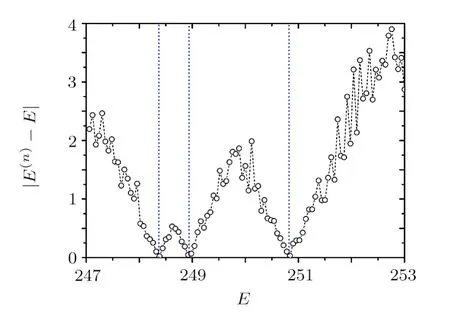
Fig.2 Variation of |E(n) −E| (circles connected by dashed lines) with E for n=5,the parameters N=300,b=100,λ=10,and E=247 + 0.06m with m=1,2,...,100.At each step of the renormalized Hamiltonian flow,30 basis states are decimated.Within the energy region shown in this figure,the original Hamiltonian has three eigenenergies with positions indicated by the three vertical dotted lines.Approximate values of the eigenenergies can be get from extrapolation of the circles close to the local minima of |E(n)−E|.
3.2 Localization of Eigenfunctions
Based on Eq.(23),the theory here can also be used in the study of properties of energy eigenfunctions ofH(0),namely,the components ofin.For this,one should first know the eigenenergyEα(0),which may be obtained by the method discussed in the previous section or by some other method.Next,one can useE=Eα(0)to construct a finite renormalized Hamiltonian flow,untilwhose dimension is small enough for direct numerical diagonalization.Then,one can perform direct numerical diagonalization for this Hamiltonian and findwhich give the corresponding components ofinby the relation (23).In this way,some information about the wavefunctione.g.,its localization properties,may be obtained.In fact,if data for the construction ofofm=1,...,nhave been stored,it is even possible to obtain all the components
We also employ the WBRM model discussed in the previous section to check the applicability of the method discussed above.Consider,e.g.,the parametersN=100,b=4,andλ=10.Hamiltonians with these parameters have localized eigenfunctions,e.g.,the one shown in Fig.3 by the solid curve.To check the validity of Eq.(23),we first diagonalizeH(0)directly and obtain its eigenenergiesEα(0)numerically.Then,we construct a(finite)renormalized Hamiltonian flowwithE=Eα(0),by making use of the method discussed in Subsec.2.4 with 10 basis states decimated at each step.Our numerical results indeed confirm the prediction of Eq.(23).An example is given in Fig.3 forn=5,which shows that the values ofagree well with the corresponding ones ofeven whenis as small as e−20.
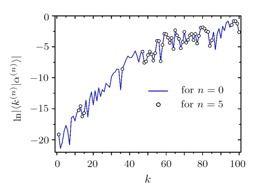
Fig.3 Values of the componentsfor n=0 and 5 in a renormalized Hamiltonian flow of .The original Hamiltonian is a realization of the Hamiltonian matrix in the WBRM model with parameters N=100,b=4,and λ=10.In the construction of the renormalized Hamiltonians,E=Eα(0) and 10 basis states are decimated at each step of the flow. and are eigenstates of H(0) and,respectively,with the same eigenenergy Eα(0).The two eigenfunctions agree well,as predicted in Eq.(23).
3.3 A Discussion of Computation Time
In this section,we give a brief discussion for the dependence of the computation time required by the method here on the dimensionNof the original Hamiltonian.This is to be compared with the corresponding dependence in ordinary direct diagonalization methods,in which the computation time usually scales asN3.
When using the method here to calculate eigenenergies,as discussed in Subsec.3.1,one first needs to choose the energy region of interest and divide the region into consecutive segments,say,to (Ns−1) segments.Then,one can take theNsends of the segments as the parameterEand construct renormalized Hamiltonian flows.Suppose at each step totallymbasis states are decimated,withm ≪N.This requires diagonalization of anm×mmatrix,which takes a time scaling asm3.After decimation of thembasis states,one obtains a new renormalized Hamiltonian and needs to calculate its new elements.(Some elements of the renormalized Hamiltonian may remain unchanged in the decimation process.) If there areM1new elements to be calculated and the time of calculating each new element scales asM2,then,calculation of the new elements needs a time scaling asM1M2.The values ofM1andM2depend on the structure of the original Hamiltonian.For example,for a 1-dimensional chain with nearest-neighbor coupling,it is possible for bothM1andM2to be quite small;on the other hand,for a full original Hamiltonian,(N2−m2) matrix elements are changed in the first step of the flow.
Suppose one performsnsteps of the renormalization procedure and at last obtains a final renormalized Hamiltonian of dimension(N−nm).Diagonalization of the final Hamiltonian needs a time scaling as (N −nm)3.Summarizing the above results,the total computation time scales asZ=Nsn(m3+M1M2)+Ns(N −nm)3,where for simplicity in discussion,we assume thatM1M2can be taken as a constant.
The method here is useful when a narrow energy region is of interest,because in this caseNsis not large.Usually,one may choose the value ofnsuch thatnmis close toN.This givesZ∼NNs(m2+M1M2/m).Comparing it withN3for direct diagonalization method,we see that the method here is more efficient ifNs(m2+M1M2/m)≪N2.In fact,the method here has another advantage,that is,it needs a relatively small memory for diagonalization.Specifically,it needs to diagonalize matrices with dimensionsmand (N −nm),respectively,which can be small even for largeN.In contrast,a direct diagonalization method usually requires a memory scaling asN2,which is much larger thanm2and (N −nm)2.
4 Conclusions and Discussions
In summary,based on the GBWPT,we propose a general method of constructing renormalized Hamiltonian flow with the energyEof interest as a parameter.Eigenenergies of the original Hamiltonian appear as (unstable) fixed points of some property of the renormalized Hamiltonian flow.WhenEis chosen as an eigenenergy of the original Hamiltonian,all the renormalized Hamiltonians in the same flow share the same eigenenergy asE,with the corresponding eigenfunctions possessing related components.we introduce a useful technique,by which an arbitrary set of basis states in the Hilbert space can be decimated in the construction of a renormalized Hamiltonian.We also discuss potential applications of the method in numerical evaluation of eigenenergies as well as in the study of localization of eigenfunctions,and illustrate them numerically in the WBRM model.In particular,by considering the scaling behavior of computation time,we find some situations in which the method here may be more efficient than the ordinary numerical diagonalization methods.
As is known,localization in the WBRM model can be related to localization in another band-random-matrix model,by making use of a renormalization technique based on the GBWPT.[48]The method discussed in this paper can be used to improve the method in Ref.[48],specifically,by partial diagonalization of the Hamiltonian in the subspace spanned by states in,without rotation in the subspace spanned by states inSα.
Finally,we give some remarks on the relation of the method discussed in this paper to some other methods of constructing renormalized Hamiltonians.The realspace renormalization-group method used in Refs.[33-34]for the one-dimensional tight-binding model with nearestneighbor-hopping,is in fact a special case of the method here,with the setincluding only one basis stateat each step of decimation.Its modified versions for 1D or quasi-1D systems,e.g.,those in Refs.[36–38],have some technical difference from the method here.A merit of the theory here is that it supplies a general approach to the construction of renormalized Hamiltonian flow,not restricted to some special types of models.
猜你喜欢
做人与处世(2022年3期)2022-05-26
文萃报·周二版(2022年4期)2022-02-14
Chinese Physics B(2019年6期)2019-06-18
侨园(2019年4期)2019-04-28
北广人物(2018年40期)2018-11-14
环球人物(2018年18期)2018-09-21
东西南北(2018年21期)2018-01-14
视野(2017年14期)2017-07-31
读者(2016年24期)2016-11-26
 Communications in Theoretical Physics2019年7期
- Communications in Theoretical Physics的其它文章
- Tunable Range Interactions and Multi-Roton Excitations for Bosons in a Bose-Fermi Mixture with Optical Lattices∗
- Scalar Tensor Cosmology With Kinetic,Gauss-Bonnet and Nonminimal Derivative Couplings and Supersymmetric Loop Corrected Potential
- Holographic Entanglement Entropy: A Topical Review∗
- Doubly Excited 1,3Fe States of Two-Electron Atoms under Weakly Coupled Plasma Environment∗
- Constraints on H0 from WMAP and BAO Measurements∗
- Hydrodynamic Stress Tensor in Inhomogeneous Colloidal Suspensions: an Irving-Kirkwood Extension∗