Fractional Angular Momentum of an Atom on a Noncommutative Plane∗

Jian Jing (荆坚), Qiu-Yue Zhang (张秋月), Qing Wang (王青), Zheng-Wen Long (隆正文), and Shi-Hai Dong (董世海)

1Department of Physics and Electronic, School of Science, Beijing University of Chemical Technology, Beijing 100029,China

2College of Physics and Technology, Xinjiang University, Urumqi 830046, China

3Department of Physics, Guizhou University, Guiyang 550025, China

4Laboratorio de Información Cuántica, CIDETEC, Instituto Politécnico Nacional, UPALM, CDMX 07700, Mexico

Abstract The mechanism of obtaining the fractional angular momentum by employing a trapped atom which possesses a permanent magnetic dipole moment in the background of two electric fields is reconsidered by using an alternative method.Then, we generalize this model to a noncommutative plane.We show that there are two different mechanisms,which include cooling down the atom to the negligibly small kinetic energy and modulating the density of electric charges to the critical value to get the fractional angular momentum theoretically.

Key words:noncommutative, fractional angular momentum, magnetic dipole moment

1 Introduction

The concept of spatial noncommutativity has a long history in physics.[1−2]It has attracted considerable attention in recent years due to superstring theories[3−5]since it arises naturally in the D-branes at the presence of background NS-NS B-field.[6−9]Fluctuations of D-branes are described by noncommutative gauge field theories.As a result, there are tremendous papers about quantum field theories in noncommutative space.[10−13]Noncommutative quantum mechanics has also been studied extensively.[14−20]The general study method is to map the noncommutative variables to the commutative ones,which satisfy the standard Heisenberg algebra by Boppshift (or generalized Bopp-shift), and then to solve dynamical equations in commutative space.[21]Exactly solvable models, such as noncommutative harmonic oscillator, Landau problem and some relativistic quantum mechanics models[22−23]are studied by using this method.The path integral formulation in noncommutative quantum mechanics has also been investigated.[24−25]Recently, Chaichianet al.studied the relativistic hydrogen atom with noncommutative corrections perturbatively and found that the degeneracy of several energy levels was lifted due to spatial noncommutativity.[26]Corrections to various quantum phases due to the spatial noncommutativity had also attracted many interests.[27−31]Interestingly, based on the path integral formulation in noncommutative space,Refs.[32−33]proposed a semi-classical effective Lagrangian to study the Aharonov-Bohm effect[34]in noncommutative space and presented explicit corrections due to the spatial noncommutativity.

The fractional angular momentum(FAM)has become a popular research topic since the early of 1980s[35−36]because of its applications both in quantum Hall effect and highTcsuperconductivity.[37−40]It has received renewed interests in recent years.[41−43]As we know, eigenvalues of the canonical angular momentum should be quantized in three-dimensional space because of the non-Abelian rotation group.However, this conclusion does not hold any more in the (2+1)-dimensional space-time since the rotation group in two-dimensional space is an Abelian one which cannot impose any constraints on eigenvalues of the canonical angular momentum.Due to the dynamical nature of the Chern-Simons gauge field and in the absence of the Maxwell term, one can realize the FAM in (2+1)-dimensional space-time by coupling a charged particle to the Chern-Simons gauge field.[44−47]Reference [48]found that it is possible to realize the FAM by coupling a cold ion to magnetic fields.This work was generalized to a noncommutative space in Ref.[49]It is argued that the FAM can also be generated by the spatial noncommutativity.[50]The purpose of this work is to realize the FAM on the noncommutative plane.Different from Ref.[49]in which the FAM is realized by a trapped charged particle on the noncommutative plane, we realize it by a trapped neutral particle, i.e., a trapped atom which possesses a permanent magnetic dipole moment in the background of electric fields.

This paper is organized as follows.For the purpose of fixing our conventions and further studies, we start from the commutative plane in Sec.2.Although this model has been investigated in Ref.[51], we shall analyze it by applying a different method.In Sec.3, we generalize the model studied in Sec.2 to the noncommutative plane.We show that there are two different mechanisms to realize the FAM on the noncommutative plane.Some concluding remarks will be given in last section.

2 The FAM in the Commutative Plane

In order to fix our convention, we re-exam the model which was proposed in Ref.[51]in this section by applying a different method.The Hamiltonian that describes dynamics of an atom with a permanent magnetic dipole moment in the background of an electric field is given by

wherem,p=−i∇,µ,c,n, andEare the mass of the atom, canonical momentum, magnitude of the permanent magnetic dipole moment, speed of light in vacuum, unit vector along magnetic dipole moment, and the electric field respectively.

Hamiltonian (1) is the non-relativistic limit of a spinhalf relativistic neutral particle, which possesses a permanent magnetic dipole moment interacting with an electric field.We assume that the atom is trapped by a harmonic potential and confined in a plane perpendicular to the magnetic dipole moment.Apart from these, two electric fieldsE=E(1)+E(2)are applied simultaneously, i.e.,

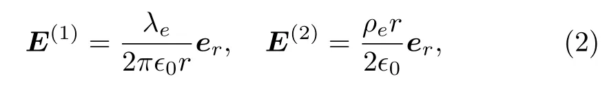
whereE(1)is generated by a long filament with a uniform chargesλeper unit length,ϵ0is the dielectric constant,ρeis the density of electric charges which is the source of electric fieldE(2),eris the unit vector along radial direction on the plane.In fact, only the electric fieldE(2)contributes to the term∇·Esince∇·E(1)=0 in the arear≠ 0 where the atom moves.Therefore, one has∇·E=∇·E(2)=ρe/ϵ0.

The Lagrangian which corresponds to Hamiltonian(1)is

Starting from this Lagrangian, Ref.[51]shows that eigenvalues of the canonical angular momentum of the reduced model which is obtained by cooling down the atom to the negligible kinetic energy, i.e., neglecting the kinetic energy term in the Lagrangian (2), will take fractional values.Here,we apply an alternative method to analyze this problem.

Observing the termn×Ein Lagrangian(3)plays the same role as the magnetic vector potential in describing a charged particle in the background of a magnetic field,it is convenient to introduce the effective vector potentialAeff=n ×E.The direction of the effective magnetic potential is parallel to the plane since the magnetic dipole moment and electric fields (2) are perpendicular and parallel to the plane respectively.As a result, the effective magnetic field which is given byBeff=∇×Aeffobviously is perpendicular to the plane.

In terms of the effective vector potential, we write Lagrangian (3) in the form

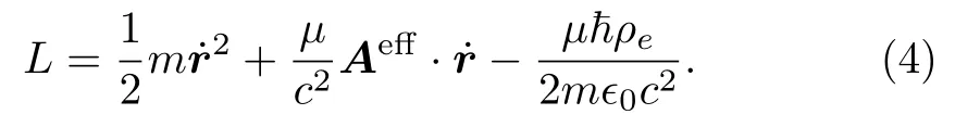
Since we only focus on the dynamics on the plane, we write the above Lagrangian as

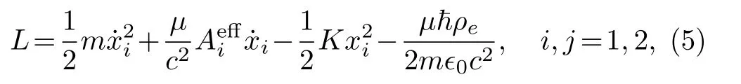
where a harmonic potential(1/2)Kx2i,which is applied to trap the atom is included and the summation convention is applied.In two-dimensional space, the effective magnetic vector potential and magnetic field are expressed explicitly as

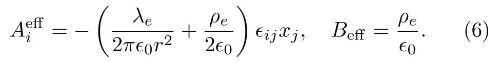
Instead of contributing to the effective magnetic field, the electric fieldE(1)only has contributions to the effective vector potential due to its topological nature.

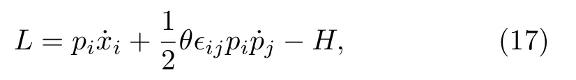
We shall show that the result in Ref.[51]can be reproduced by basing on the first-order Lagrangian(5).The first-order form of the Lagrangian (5) is

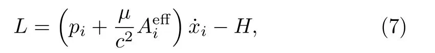
in whichHis given by

For the sake of further studies, we quantize model (7)canonically.To this end,we introduce canonical momenta(πxi, πpi)with respect to variables(xi, pi)in the standard way.They are

in which we replaceby a symmetric form(1/2)(1/2)and drop a total time derivative term in Lagrangian (7).The non-vanishing Poisson brackets among canonical variables (xi, pi, πxi, πpi) are{xi, πxj}={pi, πpj}=δij.The canonical angular momentum is defined by

Since there are no “velocities” on the right-hand sides of Eq.(9), the introduction of canonical momenta leads to primary constraints.[52]They are

where “≈” is weak equivalence, which means equivalent on the constraint surface.

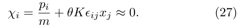
Since we are interested in the case of cooling down the atom to the limit of negligibly small kinetic energy,there are two additional constraintsχi=pi ≈0 appear in this limit.We treat all constraintsχi ≈0,ϕ(0)i ≈0,and0 on the same footing although they originate differently from model (7).We label them in a unified way as ΦI=(ϕi, ψi, χi), I=1,2,...,5,6.One must make sure whether there are secondary constraints before proceeding on.For this purpose,we apply the consistency condition to ΦI ≈0,

whereHT=H+λIΦIis the total Hamiltonian withλIbeing Lagrange multipliers.[52]

The matrix of Poisson brackets among constraints ΦI,i.e., {ΦI,ΦJ} is

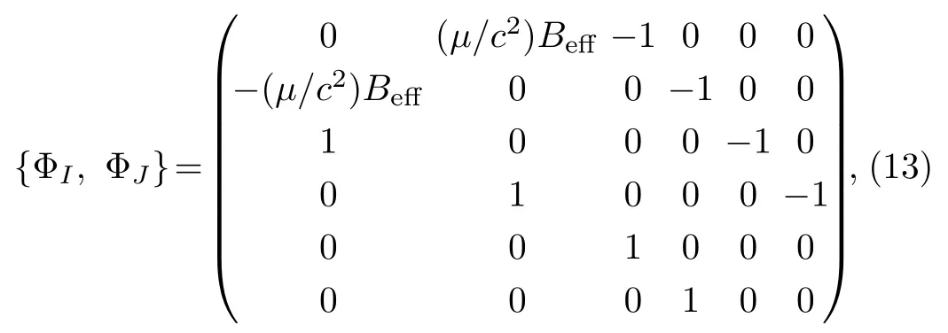
from which we can calculate the determinant of the matrix {ΦI,ΦJ}.It gives det {ΦI,ΦJ}=((µ/c2)Beff)2.Thus,the consistency condition of the primary constraints (12)can only determine Lagrangian multipliers.According to Ref.[52], there are no secondary constraints and all constraints ΦI ≈0 belong to the second class.Therefore,they can be regarded as “strong” equivalence and can be used to eliminate dependent degrees of freedom.After substituting constraints ΦI ≈0 into the canonical angular momentum (10), we get

In order to get its eigenvalues, we must know commutators between variablesxi.The classical version of commutators, i.e., Dirac brackets betweenxican be calculated according to the definition,{xi, xj}D={xi, xj}−{xi,ΦI}{ΦI,ΦJ}−1{ΦJ, xj},in which {ΦI,ΦJ}−1is the inverse of the matrix {ΦI,ΦJ}and can be written explicitly as

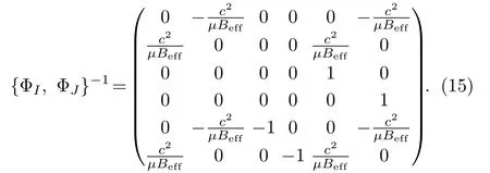
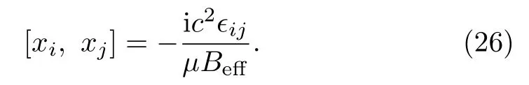
After some direct algebraic calculations, we get{xi, xj}D=−c2ϵij/µBeff.Thus, commutators betweenxiare [xi, xj]=−ic2ϵij/µBeff(in the unit of=1).

Using above commutators betweenxi, one finds that apart from a constantµλe/2πc2ϵ0, the canonical angular momentum (14) is analogous to the Hamiltonian of a one-dimensional harmonic oscillator with unit frequency.Thus,eigenvalues of the canonical angular momentum are

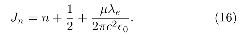
Obviously, besides the “normal” partn+ 1/2, the last term which is proportional toλecan take fractional values because of the classic parameterλe.Therefore, the eigenvalues of canonical angular momentum can take fractional values when the atom is cooled down to the limit of negligible kinetic energy.The result obtained by using this method is in accordance with previous work.[51]The advantage of this method is that it can be easily generalized to the noncommutative plane as to be shown below.

3 The FAM on a Noncommutative Plane

We now generalize above studies to the noncommutative plane.We shall show that there are two different mechanisms to get the FAM on the noncommutative plane.

The noncommutative plane is characterized by the algebraic relations

in whichθis the noncommutative parameter.It can be checked that the classical version of the above commutators can be realized by the first-order Lagrangian[25,53−54]

in whichHis a specific Hamiltonian.

There are two different ways to incorporate a magnetic field in noncommutative quantum mechanics.One is to modify the commutators between momenta directly,[14]the other is by the minimal coupling.[53]It is shown that due to the Jacobi identity,the former way is only valid for the uniform magnetic field.[54]In order to have a wider application, we choose the latter to introduce the magnetic field.The minimal coupling is achieved by substitutingpibypi+(µ/c2), i.e.,pi →pi+(µ/c2)in the first term of Lagrangian (17).Thus, the Lagrangian in our model takes the following form

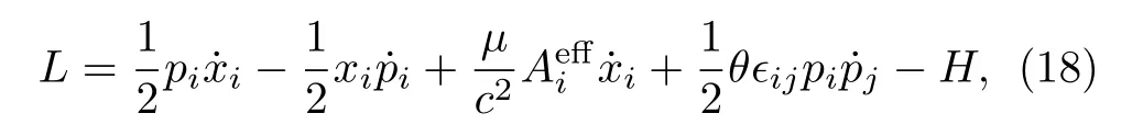
where we have symmetrized the termas (1/2)(1/2)xi˙piand dropped a total time derivative term,His given in Eq.(8).Similar to the commutative case, in order to quantize it canonically, we introduce canonical momenta with respect to variablesxi, pias

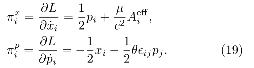
By definition, the canonical angular momentum takes the same form as Eq.(10).

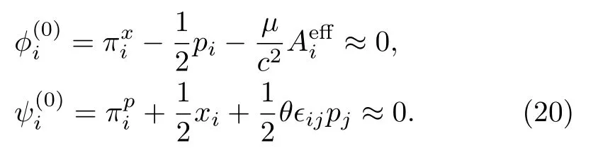
The introduction of canonical momenta (19) will lead to primary constraints which are labeled as

One must make sure whether there are other constraints besides constraints0 and0 in model (18).In doing so,we apply the consistency condition to primary constraints,

where

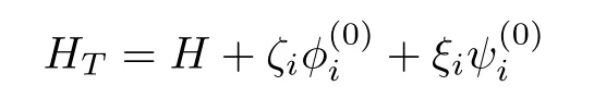
is the total Hamiltonian withζi,ξibeing Lagrange multipliers.After some algebraic calculations, we arrive at

in which

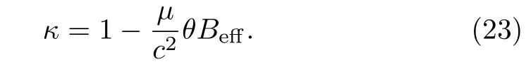
Obviously, Lagrange multipliersζi, ξican be determined providedκ≠ 0.In this case, there are no secondary constraints.On the contrary, constraint chains are not ended and the consistency condition of primary constraints will produce further constraints.We will analyze these two cases separately and show that the FAM can arise from both cases by different mechanisms.

3.1 The Case of κ≠0

In this case, there are no secondary constraints since the Lagrange multipliersζi, ξiare completely determined by the consistency condition (21).Therefore, constraint chains are ended.In order to get the FAM, we cool down the atom to the limit of negligible kinetic energy.Thus,besidesthere are two additional constraintsξi=pi ≈0.We label all constraintsin a unified way asThe matrix of the Poisson brackets among constraints ΨIis

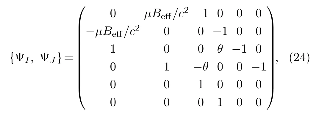
which can be verified that det {ΨI,ΨJ}≠ 0.Therefore,besides ΨI, there are no secondary constraints, all constraints ΨIbelong to the second class.Thus, they can be used to eliminate dependent degrees of freedom.

Taking constraints ΨIinto consideration, we find that the canonical angular momentum(10)reduces to the same form as Eq.(14).However,one must determine commutators betweenxiso as to get eigenvalues.The classical version of commutators betweenxi, namely, Dirac brackets betweenxican be calculated according to the definition.

The inverse matrix of {ΨI,ΨJ} is

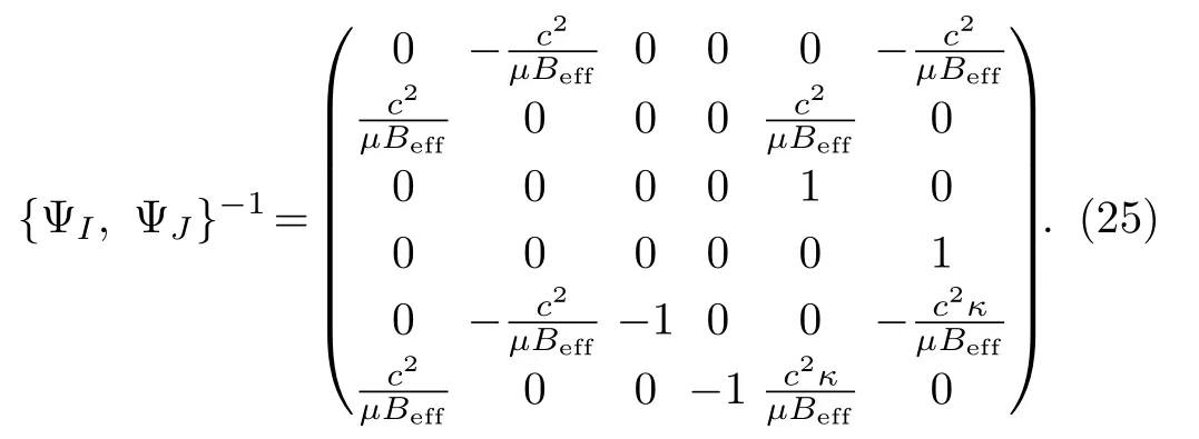
With the help of {ΨI,ΨJ}, we can calculate the Dirac brackets betweenxi.They are{xi, xj}D=−c2ϵij/µBeff.Replacing above Dirac brackets by the quantum commutators,{ , }D →(1/i)[,], we get commutators betweenxi, i.e.

Substituting the constraints ΨIinto the expression (10)and after some direct algebraic calculation, we get the canonical angular momentum.It takes the same form as Eq.(14).According to these commutators and the expression of canonical angular momentum,we get the eigenvalues of the canonical angular momentum.They take the same form as Eq.(16).This means that in the case ofκ≠0, we can cool down the atom to the limit of negligibly small kinetic energy to get the FAM from the model(18) on the noncommutative plane.

Both commutators amongxiand FAM in the commutative case are equivalent to its noncommutative counterpart when the kinetic energy of the atom is cooled down to negligibly small.This can be understood from Lagrangian(18) which implies that when the atom moves in a very low speed, the third term in Lagrangian (18), which is responsible for the spatial noncommutativity, is negligible.So, all results (including commutators among coordinates and fractional angular momentum) of the noncommutative case are equivalent to the commutative case when the atom is cooled down to the negligible kinetic energy.

3.2 Special Case κ=0

In this subsection, we analyze the special caseκ=0.This case can also be understood as the effective magnetic fieldBefftakes critical value, i.e.,Beff=Bc=c2/θµ.We will show that the FAM arises naturally in this case.

The consistency condition of primary constraints (22)show that constraint chains are not ended and there are secondary constraints whenκ=0.A straightforward calculation shows that consistency conditions(21)lead to the same secondary constraints whenκ=0.We choose the former and label them as

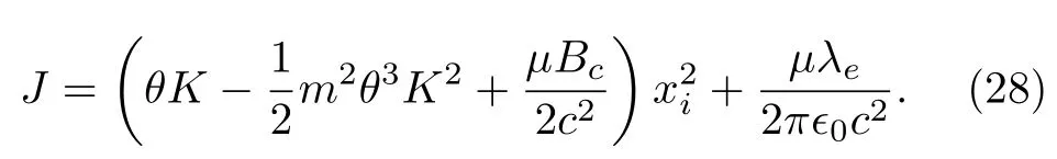
It can be checked that consistency conditions of secondary constraintsχi ≈0 does not lead to further constraints and all constraints are second class.We label these constraints asAs a result, they can be used to reduce dependent degrees of freedom in the canonical angular momentum (10).Substituting constraints (20) and(27) into Eq.(10), we get the canonical angular momentum

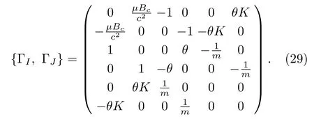
The matrix of Poisson brackets among constraints ΓIis

Its inverse is calculated as

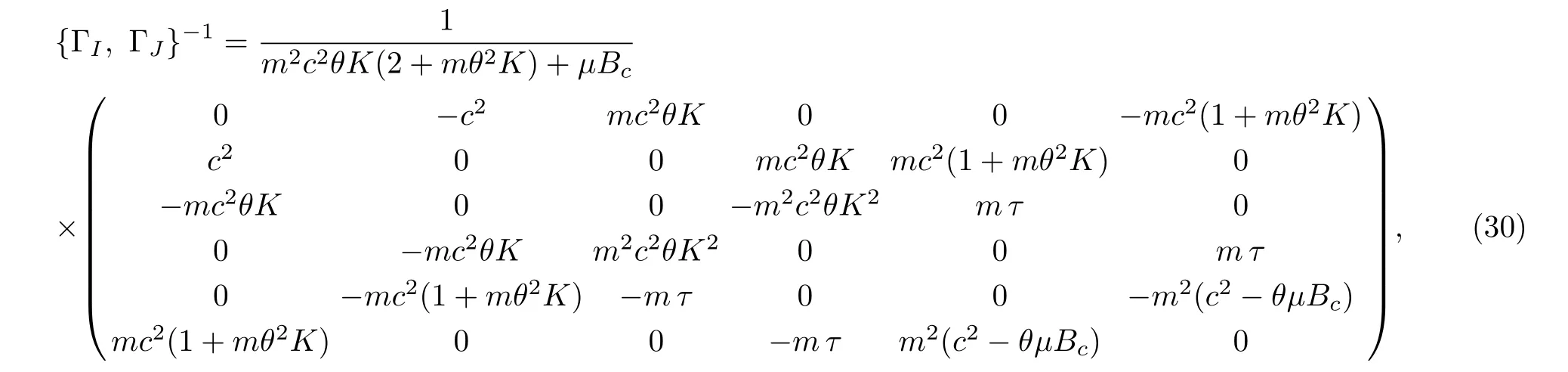
whereτ=(mc2θK+µBc).The commutators between variablesxican also be obtained as

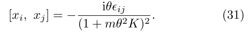
With the help of these commutators,one can obtain eigenvalues of canonical angular momentum.They are nothing but Eq.(16).It shows that the FAM appears naturally in this special caseκ=0.

4 Concluding Remarks

Based on the first-order Lagrangian(18), we study rotation properties of an atom which possesses a permanent magnetic dipole moment in the background of electric fields on a noncommutative plane.The interaction between a magnetic dipole moment and an electric field is similar with the minimal coupling between a charged particle and a magnetic field.Thus, it is convenient to introduce the effective magnetic vector potential and the corresponding effective magnetic field.Compared with previous work which realizes the FAM by charged particles, we realize it by an atom which possesses a permanent magnetic dipole moment.The present work can be regarded as a noncommutative generalization of the study in Ref.[51].

We show that there are two different ways to realize the FAM on the noncommutative plane.One is to cool down the atom to the negligible kinetic energy, the other is to modulate the intensity of the effective magnetic field to the critical value.The effective magnetic field relates the density of the electric charge byBeff=ρe/ϵ0,it means that the later way of getting the FAM is in fact, by modulating the density of the electric charges to the critical valueρe=c2ϵ0/θµ.

These two ways belong to different mechanisms.In the former mechanism,two additional constraintsχi=pi ≈0 arise during the process of cooling down the atom.These two additional constraints originate differently from the onesϕi ≈0 andψi ≈0 which originate from the singularities of the first-order Lagrangian (18).This procedure of getting the FAM is analogous to the commutative counterpart of the model (18).The latter mechanism is related to the spatial noncommutativity of the plane where the atom moves.When the intensity of the effective magnetic field approaches the critical value, the consistency condition of primary constraints will lead to two secondary constraints.These two secondary constraints play crucial roles in producing the FAM.