Evaluation of ensemble learning for Android malware family identification
2020-04-09 04:01JordanWylie谭志远AhmedAlDubai王建珍
广州大学学报(自然科学版) 2020年4期
Jordan Wylie, 谭志远*, Ahmed Al-Dubai, 王建珍
(1. School of Computing, Edinburgh Napier University, Edinburgh, EH10 5DT, UK; 2. 山西大学 商务学院/信息学院, 山西 太原 030031)
Abstract: Each Android malware instance belongs to a specific family that performs a similar set of actions and shares some key characteristics. Being competent to identify Android malware families is critical to address security challenges from malware and the damaging consequences. Ensemble learning is believed an improvement to solve computational intelligence problems by strategically combining decisions from multiple machine learning models. This paper, thus, presents a study of the application of ensemble learning and its effectiveness in Android malware family identification/classification against other single-model-based identification approaches. To conduct a fair evaluation, a prototype of ensemble learning based Android malware classification system was developed for this work, where Weighted Majority Voting (WMV) approach is used in this prototype to determine the importance of individual models (i.e., Support Vector Machine, k-Nearest Neighbour, ExtraTress, Multi-layer Perceptron, and Logistic Regression) to a final decision. The results of the evaluation, conducted by using publicly-accessible malware datasets (i.e., Drebin and UpDroid) and the recent samples from GitHub repositories, show that the ensemble learning approach does not always perform better than single-model learning approaches. The performance of the ensemble learning based malware family classification is heavily influenced by several factors, in particular the features, the values of the parameters and the weights assigned to individual models.
Key words: Android malware; family identification; static analysis; ensemble learning
1 Introduction
Android took the largest market share in the mobile operating system (OS) market in 2012 for the first time ever and which has been continuously growing since then, as shown in Fig.1 that was drawn based on data from[1]. As of May 2019 Android had 2.5 billion monthly active devices[2]. Due to this popularity the threat of malware, which is defined as software that has malicious intent[3-4], increases. Every malware sample belongs to a family of malware that all have a similar set of characteristics, in regards to how they are implemented and their goals. Android malware family identification assists in the identification of steps that could be taken to overturn any damage that has been caused by a specific malware sample[5]. This shows that techniques, being able to identify malware families efficiently and effectively, are vital.

Fig.1 iOS and Android mobile OS market share[1]
This paper, therefore, develops an approach to identify Android malware families, in which an ensemble learning algorithm, termed weighted majority voting, is applied to build the malware family classifier. The ensemble learning approach was chosen over other approaches because they perform well when applied to real world issues, improve accuracy, and handle the problems of concept drift and unbalanced data[6]. To fairly evaluate our proposed ensemble learning based malware family identification approach, publicly available evaluation datasets are used. However, the majority of recent related approaches were evaluated on datasets that are out of date which makes it difficult to evaluate how well these related approaches would perform on samples from the current Android malware landscape. This also causes issues when providing comparisons between our proposed approach and these related approaches. To solve these issues, multiple datasets, including commonly-used and recently-discovered malware samples, will be used. Through this research, we aim to answer two main questions defined below.
(1) How does our ensemble learning approach for Android malware family identification compare to other related single-model-based Android malware classification approaches?
(2) How effective is our approach developed in classifying recent Android malware into their respective families?
1.1 Impact
This work will have an impact on the general public, providing security experts with a weapon to respond to new variants of known malware families effectively which should ultimately result in the competence to define their impact and the steps that could be taken to mitigate any damage caused.
In addition, the evaluation approach developed in this work will inform how a varied set of classifiers perform while tackling the family identification problem, which will guide the development of new defense approaches.
1.2 Paper organisation
The rest of this paper is organised as follows.
• Section 2: Provides a relevant technical background, including the structure of an Android application, the different malware analysis evaluation techniques, the evaluation metrics and datasets;
• Section 3: Presents a critical review into recent related works;
• Section 4: Informed by Section 2, this section proposes a viable ensemble learning approach with an aim to answer the questions defined in Section 1;
• Section 5: Critically evaluates the proposed approach making use of multiple metrics discussed in Section 4;
• Section 6: Concludes the paper and evaluates how well the questions defined in Section 1 were answered. This section will also provide potential future work.
2 Technical background
2.1 Android application structure
An Android Package (APK) is an archive file that contains various files and directories[7], defined in Table 1.
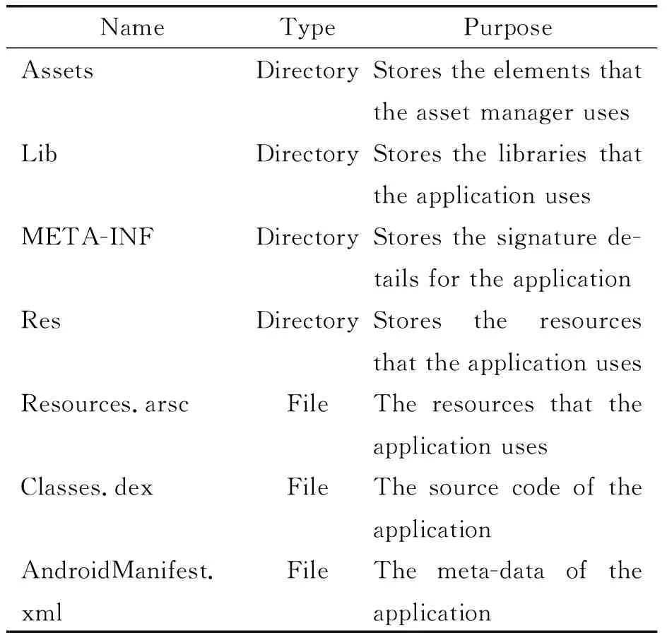
Table 1 Contents of an APK file[8]
There are four different app components that are used by an Android application to provide the system or a user to enter itself. These are activities, services, broadcast receivers, and content providers[7,9]and they are defined in Table 2.

Table 2 Types of Android components[7,9]
The activities, services and broadcast receivers are activated by an Intent, which is a messaging object that an Android application use to request an action from another components. A request can be either explicit (where a specific app component will be requested) or implicit (where, in contrast, a type of components will be requested instead). Recent research[9]shows “broadcast receivers” app component was used more often than the other components by malware, and the same components tended to be used across the malware variants of the same family as malware creators reused some of the developed functions.
To protect user privacy, app permissions are supported by Android, who categorises the permissions into three different groups, namely normal, signature, and dangerous permissions[10]. The 36 normal permissions are low-risk and automatically granted during installation[10-11]. The 29 signature permissions, in contrast, require the requesting and the consuming Android application must be the same[10-11], and two special signature permissions are considered sensitive and should not be used by the majority of applications[10]. The 28 dangerous permissions controlling access to data and private resources, require user confirmation[10].
2.2 Malware analysis and anti-analysis techniques
Malware analysis aims to understand the working and intention of malware in order to identify any infected devices and files[12]. This is commonly done through static analysis and dynamic analysis. No execution of the malware of interest is required during the static analysis, whereas the dynamic analysis is in the opposite[12].
On the other side, to hinder the analysis, anti-analysis techniques have been used in malware creation[13].
Techniques, such as string encryption and encoding, dynamic loading, native payloads and reflection, help creators to produce evasive malware to bypass dynamic analysis[13-15].
2.3 Machine learning
Several metrics have been commonly used by researchers and practitioner to evaluate the effectiveness of trained Machine Learning (ML) models. From the four most basic metrics[16-17], the following advanced metrics shown in Table 3 can be derived.
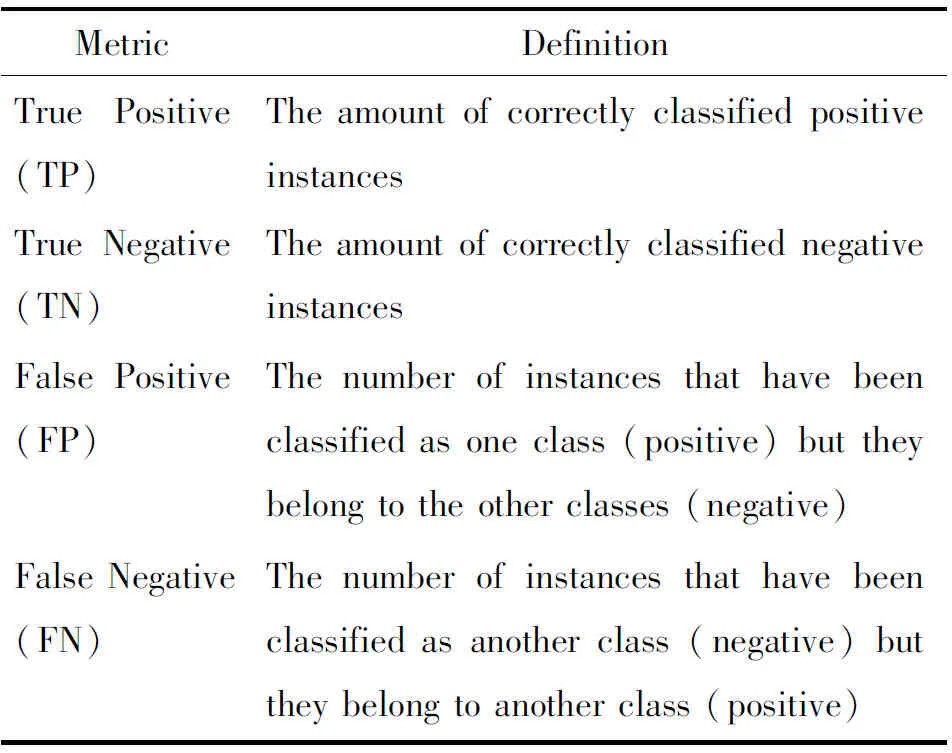
Table 3 Main machine learning metrics[18]
(1)Accuracy: TheAccuracyis the ratio of instances that were classified correctly[16]and is calculated using Equation 1. This metric is effective when classes are balanced. As such, this metric only renders a fair evaluation during the afore-mentioned condition.
(1)
(2)Recall: TheRecallshows how many relevant instances were classified into a specific class[11, 16, 17, 19]and is calculated using Equation 2.
(2)
(3)Precision: ThePrecisionis the ratio of instances that have been classified correctly against all other instances that were correctly or incorrectly classified to that class[18-19]. This is calculated using Equation 3.
(3)
(4)F1-Score: TheF1-Scorecan also be used to evaluate the performance of a model. This is the harmonic mean between the recall and precision metrics[17, 20]and is calculated using Equation 4.
(4)
These four advanced metrics will be used in our evaluation.
2.4 Datasets
These are the Android Malware Genome Project (AMGP), Drebin, Android Malware Dataset (AMD), UpDroid, Android PRAGuard, AndroZoo, and samples obtained from GitHub.
(1)AMGP: The AMGP is a dataset that has been used in previous Android malware family identification approaches[5,15], however it has now been discontinued[13, 21]. The dataset contained a total of 1 260 samples that were gathered between August 2010 and October 2011 from multiple marketplaces including the official Google marketplace[22].
(2)Drebin: The Drebin dataset[23]is another widely used dataset that has been used by various approaches[5, 15]. This dataset has a total of 5 560 samples which were gathered between August 2010 and October 2012 from multiple sources including the Google Play Store, third party marketplaces, and the AMGP[23].
(3)AMD: The AMD[13]contains 24 560 samples which were obtained from 2010 to 2016 from the Google Play Store, third party security companies, and VirusShare. Each of the samples is associated with a family.
(4)UpDroid: UpDroid[24]contains 2 479 samples, 50% of which were collected from 2015 onwards. Each of these samples had to be flagged as malicious by at least 20 anti-virus software from VirusTotal. The family name was also derived from the VirusTotal results.
(5)Android PRAGuard: The Android PRAGuard dataset[14]contains malware from the AMGP and the Contigio dataset. These samples were also obfuscated to form this dataset.
(6)AndroZoo: The AndroZoo dataset[25]that contains millions of benign and malicious applications. These were obtained through the use of crawlers which were obtained from multiple sources including the Google Play Store, third party marketplaces, torrents, and the AMGP.
(7)GitHub: There are also multiple repositories on GitHub[26-27]which have more recent samples. The samples obtained from this source would have to be analysed further due to its unreliability.
Among these seven reviewed datasets, some are more appropriate than the others to be used to evaluate our proposed malware family identification approach. Although the AMGP has been used in several research works. It is outdated and not accessible anymore. The Drebin dataset has also been used to evaluate a significant number of detection approaches, but it is outdated and would not give a real representation of current Android malware too. Similarly, the AMD is an outdated dataset, which however is large in size and could help establishing a better overview of model performance. A more recent dataset. The UpDroid dataset, however, small and has not been used as much. Apart from these old datasets, there are still a few more recent perspective datasets available. The Android PRAGuard dataset is more representative of the current malware landscape as these samples were modified for obfuscation purposes. The AndroZoo dataset could also be used as it is a large dataset in spite of containing benign samples. Last but not least, recent samples from GitHub are accessible but these would not be as reliable as the other datasets mentioned. There are two main criteria to select an evaluation dataset.
(1)Being able to provide a comparison with other family identification approaches.
(2)Being able to show how the approach of interest will perform with more recent samples.
Based on the above criteria, three datasets are selected for this research work. They are the Drebin dataset, UpDroid, and samples obtained from GitHub.
3 Related works
Android malware family identification has been widely studied. These related approaches differ themselves from each other by the features used in analysis. The following paragraphs review several key recent related approaches. The quantified evaluation results are summarised in Table 4.
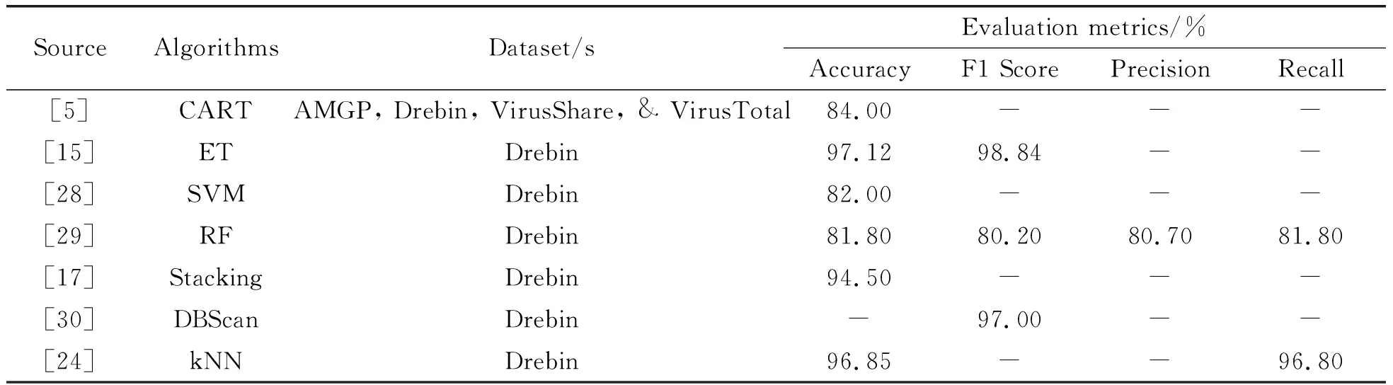
Table 4 Summary of family identification approaches
3.1 Approaches using static features
RevealDroid[5]uses static features in malware family classification. Its main aim was to be resilient to obfuscation techniques. The Classification and Regression Trees (CART) algorithm was applied and a total of 1 054 features were used to build the classifier. This approach was evaluated using a total of 27 979 samples gathered from the AMGP, the Drebin dataset, VirusShare, and VirusTotal. This approach achieved an accuracy of 84%. Whereas no other metrics have been used to evaluate the performance of this approach which makes it difficult to ascertain how well this approach has performed. This is due to the fact that accuracy does not provide a good indication of how well an approach performed when the classes are unbalanced[16, 19].
Similarly, DroidSieve[15]made use of the ExtraTrees (ET) algorithm and static features in order to infer Android malware families. Four datasets including the AMGP, Drebin dataset, Marvin dataset, and Android PRAGuard were used to evaluate DroidSieve. DroidSieve achieved outstanding performance (i.e., an accuracy of 98.12% and an F-measure of 97.84%) on the Drebin dataset and (i.e., an accuracy of 99.15%) on the AMGP and Android PRAGuard dataset. However, The main issue with this approach is that the Android PRAGuard dataset is a obfuscated version of the AMGP and the Contagio dataset[14]. These obfuscated samples are not samples found in a real life environment.
3.2 Approaches using dynamic features
To characterise malware and its runtime behaviour, dynamic features of the malware of interest are extracted from a live environment. A recent research, conducted by Massarelli, et al.[28], made use of Support Vector Machine (SVM) to build a malware classifier with the dynamic features. The Drebin dataset was utilised to evaluate this SVM-based classifier. A70-30 train-test split was applied, and stratified 5-fold cross validation was executed for 20 times. Their approach was able to obtain a mean accuracy of 82%. Although the precision and recall were reported, however, these were calculated for each individual class label (family).
CANDYMAN[29]involves dynamic features and various classifiers including the Random Forest (RF). This approach was evaluated using the Drebin dataset, from which a total of 4 442 samples from 24 families were taken for evaluation after removing the malware families with fewer than 20 samples. Features of the malware samples were extracted using a Markov chain from the raw features provided through emulation. With the RF classifier, CANDYMAN was able to achieve an accuracy of 81.8%, an f-measure of 80.2%, 80.7% precision and 81.8% recall.
EnDroid[17]is another approach that made use of dynamic features as well as the stacking classifier. It achieved an accuracy of 94.5% when evaluated against the top 20 malware families with 4 446 samples from the Drebin dataset.
3.3 Approaches using hybrid features
Some recent work attempts to take advantages of both static and dynamic features. EC2[30], for example, uses both types of features to train the RF and DBScan classifiers. EC2 is again evaluated using the Drebin dataset, from where the malware samples could not without issues were discarded. The EC2 with the DBScan algorithm achieved a micro f-measure of 76% and a macro f-measure of 97%.
UpDroid[24]is another hybrid-feature approach equipped with three algorithms, namely k-Nearest Neighbors (kNN), RF, and J48. Alongside with the Drebin dataset, a dataset of 2 479 collected samples was used to evaluate the UpDroid. The samples were executed in an emulated environment for 15 minutes to obtain the dynamic features. Using the newly collected dataset and the kNN algorithm, UpDroid was able to achieve an accuracy of 96.37%, a recall of 96.4% and a false positive rate of 0.2%. On the Drebin dataset, UpDroid achieved an accuracy of 96.85%, a recall of 96.8%, and a false positive rate of 0.3%. This approach has been tested on more recent samples, however the limitation of this approach is the dynamic features used. To extract these dynamic features from the newly collected dataset would take at least 25 days to dynamically analyse every sample.
Overall, the Drebin dataset was most popular and used to evaluate all the reviewed malware classification approaches. Only UpDroid[24]was evaluated against a more up-to-date dataset. In addition, these approaches were all evaluated with varied metrics which makes it difficult to compare with the approach developed in this paper.
4 Methodology
This section defines the process of preparing and organising the datasets, analysing the samples, and defining and evaluating the family identification model. The methodology is summarised in Fig.2.
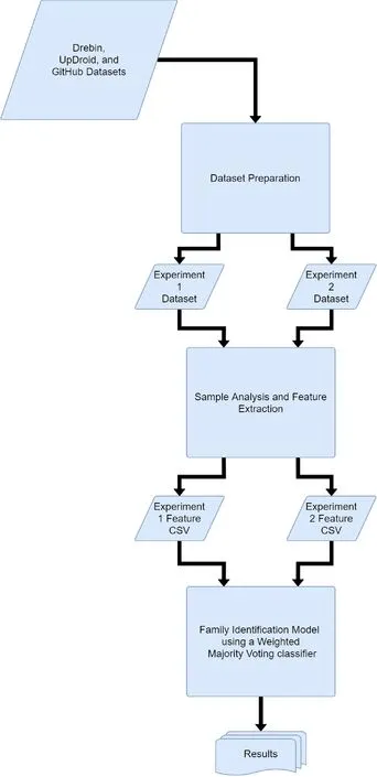
Fig.2 Overview of the methodology
4.1 Dataset selection and preparation
The datasets were chosen and obtained first. This resulted in a total of 3 datasets being chosen which aimed to answer the research questions stated in Section 1. These datasets are the Drebin dataset[23,31], the UpDroid dataset[24], and samples that were obtained from GitHub[26-27]. These datasets will be split into two experimental datasets. The first experimental dataset contains the samples from the Drebin dataset and will be used to answer our research question 1; the second experimental dataset contains samples from the UpDroid dataset and those collected from GitHub by us, and this second experimental dataset will be used to answer our research question 2.
To prepare the experimental datasets, all the samples are first organised in a similar manner and then assigned to their respective experimental datasets. Due to the nature of the GitHub samples additional analysis was carried out on those samples. Similar to the sample preparation approach introduced in Ref.[24], only the samples, discovered before May 2019, is kept to ensure they can be correctly recognised by a predefined number (e.g., 20) of major anti-virus scanners. The test results from AVClass, a Python tool to tag malware samples with their respective family label, is then used to build a ground truth of the family labels of the malware samples.
4.2 Feature extraction
To extract various static features shown in Table 5 for each sample, AndroGuard, a Python library, is used. The extracted features of the samples are stored in a CSV file. If none of these features can be extracted from a sample, then it is discarded.
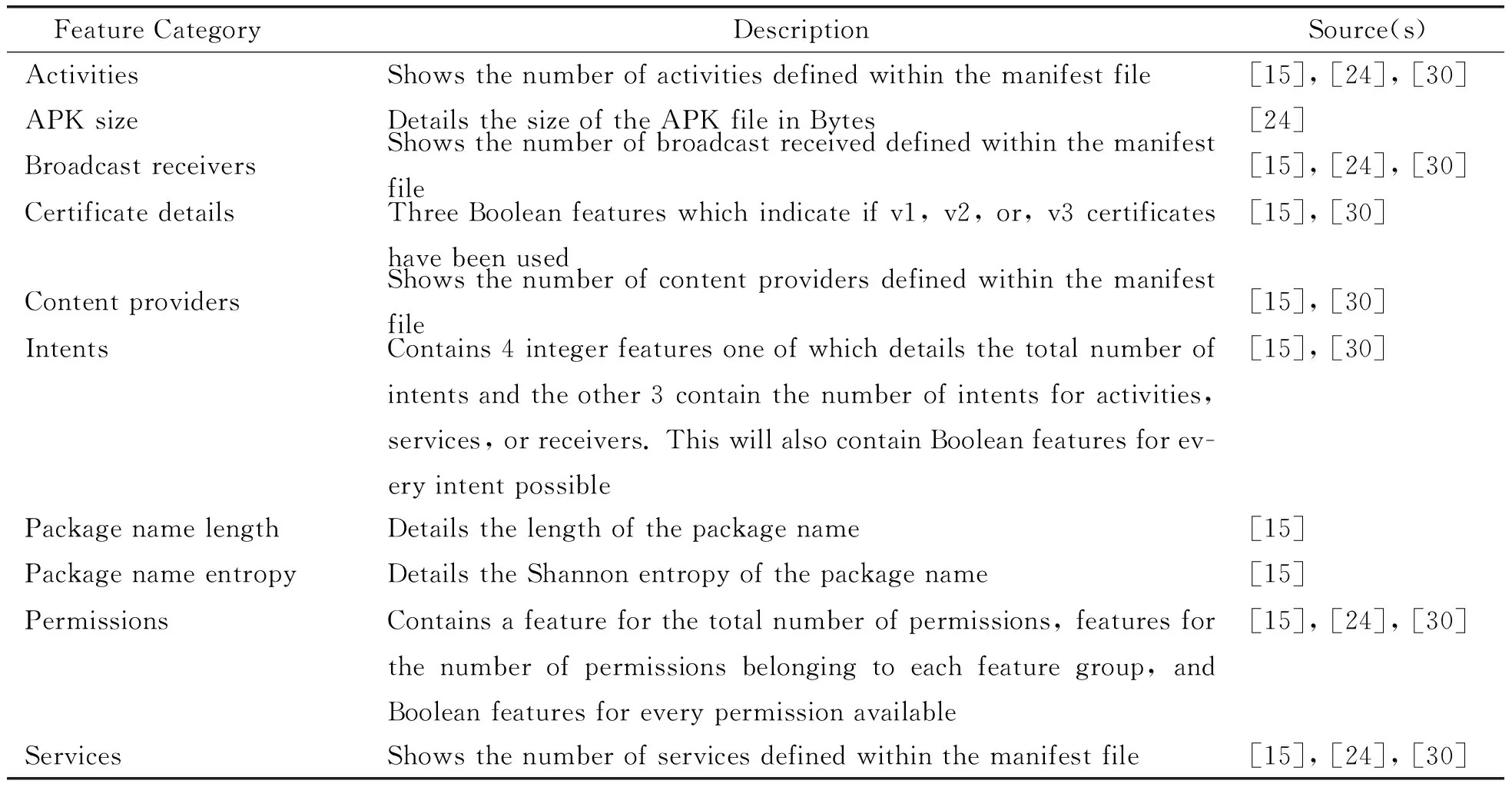
Table 5 Static features used in this project
4.3 Family identification
The family identification process steps include data preprocessing, hybrid feature selection, establishment of ensemble learning based malware classification, as well as hybrid-parameter selection. The details of these steps are discussed in the subsections below.
4.3.1 Data preparation
The malware family identification begins with data preprocessing. Given a sample setX(defined in Equation 5) that contains s samples with c features, and a respective label setY(defined in Equation 6), the training datasetDis defined as Equation 7.
Any families having fewer than 5 samples are removed when proceeding with a 5-fold cross validation. The non-Boolean features are then normalised to avoid the ML models from being biased by the features with large values. The Boolean features are not normalised as to keep the property of those features.
(5)
(6)
D=(Y|X)
(7)
where:
s=The number of samples
c=The number of features
4.3.2 Hybrid feature selection
To reduce both the noise in the data and the complexity of computation, feature selection is carried out at this stage. Hybrid feature selection is recommended as exploiting the advantages of both wrapper and filter methods. On one hand, filter methods are not prone to bias and are more time-efficient but do not always improve the effectiveness of a model[32]. On the other hand, wrapper methods usually improve the effectiveness of a model but are time-consuming[32]. As such, it would be wise to first apply a filter method.
In this work, a correlation-based feature selection, namely Pearson’s correlation as shown in Equation 8[33], is in use. The respective algorithm is defined in Algorithm 1 which removes any features having a correlation greater than 0.8 or less than -0.8. The reason that these values should be chosen is because they indicate a close relationship between the two features[34].
(8)
where:
ρx,y=The Pearson’s correlation between variablesAandB
μA=The expectation ofA
μB=The expectation ofB
σA=The standard deviation ofA
σB=The standard deviation ofB
Algorithm 1 Correlation-based feature selection
Require:Xfeature set,cfeature count
forx,yinXdo
CFx,y←ρx,y
end for
InitialisecorrF{Empty list that will contain highly correlated features}
InitialiseremF{Empty list that will contain features to be removed}
f← list of features
fori=1 tocdo
forj=i+1 tocdo
ifCFi,j<-0.8‖CFi,j>0.8 then
corrF∪{fi,fj}
end if
end for
end for
freqs← list of corrF sorted by frequency
forfeature,freqinfreqsdo
forCFTincorrFdo
iffeatureinCFT&& not inremFthen
remF∪feature
removeCFTfromcorrF
end if
end for
end for
Remove features fromXthat are inremF
returnX
For the wrapper method, the Recursive Feature Elimination (RFE) algorithm with random forest as an estimator is then used. This works by training a classifier, random forest in this case, to obtain a rank of each feature. Once each feature has a rank, the lowest one is removed, this is repeated until the desired number of features is met[35]. The number is set to 100 in this work. Once the features have been selected, these can then be saved to a new CSV file if required.
4.3.3 Establishment of malware family identification using ensemble learning with weighted majority vote
Ensemble learning is used at this stage to build an identifier to classify malware samples. The weighted majority voting mechanism is applied to strategically generate and combine models in the fashion of ensemble learning to solve this classification problem. The ML algorithms used to generate these models are SVM, kNN, ET, Multiplayer Perception (MLP) and Logistic Regression (LR). These ML algorithms have been chosen for their popularity in related research.
(1)SVM: The SVM classifier is a kernel method algorithm[36]which aims to find the hyperplane that splits the dataset into two classes. Due to this being a multiclass problem a one-vs-rest approach will be taken, where one class is split from the other classes and the class that has the largest distance from the hyperplane is the one that is predicted[36].
(2)kNN: The kNN classifier predicts the class label by looking at thekclosest samples and is assigned the class label that appears the most[37]. This is known as a lazy algorithm because of the fact that it does not have a training stage[37].
(3)ET: The ET classifier is similar to the Random Forest classifier used during the wrapper feature selection in that both of these algorithms are ensembles of trees[38]. The difference is that ET makes use of random attributes and cut point values to identify how a node is split[38].
(4)MLP: The MLP classifier is a feed-forward neural network that uses a set of neurons, in the form of at least one hidden layer which are connected using weights[39]. The weights are altered during training in order to identify the correct weights that will identify the correct class label[39].
(5)LR: The LR classifier aims to identify the relationship between a feature set and a class label[40]and tends to not over fit as much as other classifiers[41]. Like SVM, LR is a binary classifier but it is possible to use it to handle multiclass problems using a one-vs-rest approach[42].
To build the ensemble learning based classification approach, the hyperparameters for each of the five chosen classifiers need to be carefully selected. A randomised searching algorithm[43]is applied to pick 10 sets of random parameters and identify the best parameters. The randomised searching algorithm was chosen as its unique properties: (a) a budget can be chosen independent of the number of parameters and possible values; and (b) adding parameters that do not influence the performance does not decrease efficiency.
The weights for each individual classifier is then calculated using an approach similar to the approach proposed in Ref.[41] where the accuracy of each individual classifier is calculated and divided the sum of the accuracies of the individual classifiers. In this work, the F1-score is used instead due to the fact that accuracy does not perform as well with unbalanced classes[16, 19]. Our improved weighting approach is defined by Equation 9 and Algorithm 2.
(9)
where:
cis the c-th individual classifier
Wcis the weight of the c-th individual classifier
F1cis the F1-score of the c-th individual classifier
Algorithm 2 F1-score based weighting
Require: A list of classifiers {C1,C2, …,Cn}
n← the number of classifiers;Wis an empty weight set
fori=1 tondo
c←Ci
W∪{Wc}
end for
returnW
Once the initial candidate set of weights,W, is settled, our proposed malware family identifier based WMV, defined in Equation 10, is evaluated using 5-fold cross validation, where the ensemble model is trained and weights are tuned. Evaluation Metrics, including accuracy, macro F1-score, macro precision, macro recall, and macro AUC, are used alongside a macro ROC curve.
(10)
where:
yis the predicted class of samplex
mis the number of classifiers
Cjis the j-th classifier
wjis the weight of the j-th classifier
Ais the set of unique class labels
In order to cater an insight into the types of features that are significant for malware family identification, XGBoost Feature Importance Scores are calculated and the top 20 most important ones are plotted for each experimental dataset. Following the above-introduced process, the experimental results can be reproduced.
5 Evaluation results and analysis
Two experiments were conducted and the results are presented in this section. The main goal of the first experiment is to provide a comparison between our ensemble learning based malware family identification approach and other non-ensemble learning based approaches. The second experiment is to evaluate how well our proposed approach performs on recent malware samples.
5.1 Evaluation results of ensemble learning and its sub-models
This section delivers the first evaluation of our proposed ensemble learning based malware family identification approach. The performance of the ensemble learning based approach and its sub-model are shown in Table 6. As can be seen from Table 6 the ET and kNN models outperform the proposed ensemble learning based approach, WMV, on the first experimental dataset. This could be due to the limited variation between the weights of the individual classifiers which means that all classifiers were treated equally.

Table 6 The results of the first experimental dataset %
Table 7 shows that the proposed ensemble learning based approach, WMV, does outperform the models in terms of F1-score and precision on the second experimental dataset. However, it is not as good as ET with regard to the accuracy and recall. These shortfalls could potentially be improved through further research into weighting calculations.
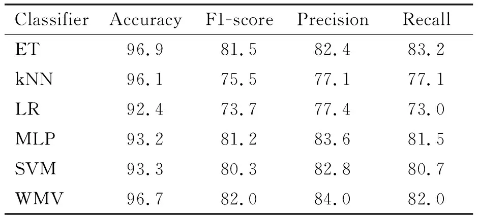
Table 7 Experiment 2 results %
5.2 Comparison between the proposed ensemble learning based malware family identification approach and other approaches
In order to answer research question 1, a comparison between our ensemble learning based approach (i.e., WMV) and other approaches[15, 17, 24, 28-30]is presented in this section. The different approaches were all evaluated using the same dataset. The evaluation results are shown in Table 8 which details the approaches, the types of features used, and the metrics used to evaluate each approach. These results show that our approach outperforms two out of the three approaches using dynamic features and falls marginally behind the other approaches using static and hybrid features. The reason for this could be due to the reduced feature set. If the feature set was increased and non-linear filter methods were used, there would be a chance that these results could improve at the expense of time. It may also be beneficial to obtain the evaluation scripts for these related approaches. This would provide the ability to evaluate the related approaches using the exact samples as although each of these approaches used the Drebin dataset, certain samples were removed which might impact the results.

Table 8 Comparison with other approaches that used the Drebin dataset %
5.3 ROC curves
As can be seen from Fig.3 the performance of the model using older samples is not perfect which show that only 59% of the time the model would classify a sample correctly. This could be due to various reasons including the fact that the dataset had a total of 83 different labels with only 100 different features to differentiate each of them.
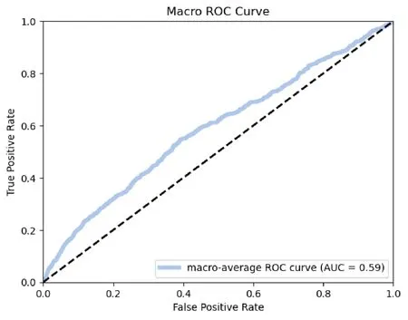
Fig.3 Experiment 1 macro-average ROC curve
The performance in experiment 2 was significantly better as can be seen in Fig.4 which shows that 75% of the time the model will classify a sample correctly. This further consolidates the above theory as although the dataset is half the size of experiment 1, it only has a total of 24 families.

Fig.4 Experiment 2 macro-average ROC curve
5.4 Feature importance
Fig.5 and Fig.6 provide the ability to differentiate between which features are important for older samples when compared to newer samples. It can be seen that in general the most important features for more recent samples are increasingly varied as well as some new features (e.g., the signature scheme) added to the list of the top 20.

Fig.5 Experiment 1 top 20 features
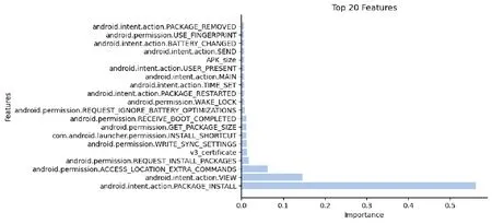
Fig.6 Experiment 2 top 20 features
6 Conclusion
This paper set out to evaluate ensemble learning for malware family classification. To understand the impact of ensemble learning on decision making and its performance in comparison with other non-ensemble learning based malware classification approach, a prototype of ensemble learning-based malware family classification was developed in this paper. The weighted majority voting approach is used in this prototype to determine the importance of individual models to a final decision. The evaluation was conducted using well-known, publicly-available datasets (i.e., Drebin and UpDroid) and the recent malware samples collected from GitHub repositories.
The evaluation results show that the prototype of ensemble learning based malware family classification outperforms almost all opponents using dynamic features, but marginally behind others using static or hybrid features. The ROC curves show the the prototype has 75% chance being able to distinguish the families of the samples in the second experimental dataset.
The results imply that the type and quality of features have significant impact on the decision; the randomised searching algorithm does not guarantee optimal selection of parameters. The proposition that ensemble learning outclassed single-model-based learning holds only if the weights of individual models are well tuned. Further investigation is sought to further confirm these implications.
猜你喜欢
电影文学(2021年17期)2021-10-14
支部建设(2021年18期)2021-08-20
发明与创新(2021年17期)2021-07-05
作文评点报·低幼版(2020年42期)2020-12-14
意林(儿童绘本)(2020年1期)2020-02-14
山西大学学报(哲学社会科学版)(2019年4期)2019-07-25
支部建设(2016年3期)2016-11-27
支部建设(2016年12期)2016-04-12
支部建设(2016年6期)2016-04-12
小学生作文·小学低年级适用(2016年1期)2016-03-07