
Path planning for moving target tracking by fixed-wing UAV
2020-07-02 03:16SonglinLioRongmingZhuNiqiWuTuqeerAhmedShikhMohmedShrfAlmetwllyMostf
Defence Technology 2020年4期
Song-lin Lio , Rong-ming Zhu ,*, Ni-qi Wu , Tuqeer Ahmed Shikh ,Mohmed Shrf , Almetwlly M. Mostf
a School of Electro-Mechanical Engineering, Xidian University, Xi’an 710071, China
b Institute of Systems Engineering, Macau University of Science and Technology, Taipa, 999078, Macau
c Electrical Engineering Department, College of Engineering, King Saud University, Riyadh 11421, Saudi Arabia
d Industrial Engineering Department, College of Engineering, King Saud University, P.O. Box 800, Riyadh 11421, Saudi Arabia
e College of Computer and Information Sciences, King Saud University, P.O. Box 800, Riyadh 11421, Saudi Arabia
f Faculty of Engineering, Alazhar University Cairo, Egypt
Keywords:Bearing angle Fixed-wing UAV Laser designation Moving target tracking Path planning
ABSTRACT For the automatic tracking of unknown moving targets on the ground, most of the commonly used methods involve circling above the target.With such a tracking mode,there is a moving laser spot on the target,which will bring trouble for cooperative manned helicopters.In this paper,we propose a new way of tracking, where an unmanned aerial vehicle(UAV) circles on one side of the tracked target. A circular path algorithm is developed for monitoring the relative position between the UAV and the target considering the real-time range and the bearing angle.This can determine the center of the new circular path if the predicted range between the UAV and the target does not meet the monitoring requirements.A transition path algorithm is presented for planning the transition path between circular paths that constrain the turning radius of the UAV.The transition path algorithm can generate waypoints that meet the flight ability. In this paper, we analyze the entire method and detail the scope of applications. We formulate an observation angle as an evaluation index. A series of simulations and evaluation index comparisons verify the effectiveness of the proposed algorithms.
1. Introduction
Helicopters are widely used in military and civilian fields because of the ease with which they can take off and hover,but they are also vulnerable to hidden targets on the ground. The miniaturization and accuracy of sensors allow unmanned aerial vehicles(UAVs)to carry a large number of them and become an information acquisition and guidance platform. In the process of cooperative helicopter operation, UAVs often need to perform tasks such as reconnaissance, laser designation, and guidance [1] to ensure the helicopters’safety and the effectiveness of the task.The continuous monitoring and designation of a non-cooperative moving target on the ground are challenging tasks for a UAV.In order to continuously monitor and track a target,multiple UAVs are usually employed.In Ref.[2],Zhao et al.introduce a decision making algorithm based on distributed multi-agent partially observable Markov decision processes (MPOMDPs). A group of UAVs is used to track multi-target.For a single target, the use of multiple UAVs increases task load.Using a single UAV would be ideal. More studies on UAV target tracking are reviewed in Section 2.
In the case of UAV-assisting helicopter operations, a UAV is not only required to track a target but also to laser-designate the target continuously. For the former, there are no major problems in the existing work, but no direct method has been found for the latter task. In a conventional tracking process, a control law does not constrain the orientation of a UAV relative to the target.This brings about a difficult problem for the helicopter: the UAV appears at different directions relative to the target at different time instances,and the laser is reflected in all directions.Therefore,constraints on the bearing angle must be added to solve this problem.
To add these constraints, this paper proposes a new tracking method:the UAV and the target on a single side.Our strategy is as follows:
· If the target is stationary or moving in a small range, the UAV moves along a circular path.
· If the predicted distance between the UAV and target exceeds a certain range,we calculate a new circular path by a circular path algorithm to re-meet the monitoring requirements.
Monitoring requires that the distance between the UAV and the target should be within a certain range.The circular path algorithm based on adaptive control decides the real time distance and continuously calculates a new circular path that satisfies monitoring requirements. After that, a transition path algorithm will generate a transition path to guide the UAV to a new circular path by considering the continuous nature of the curvature.If there is no new circular path center, the transition path algorithm is not activated and the UAV needs to circle the target on the same side for monitoring and designation only.
The target speed with which the entire planning algorithm can cope is not a specific value but is a ratio relationship determined by the monitoring range and the speed ratio between the UAV and the target.Therefore,a range of restrictions determines the application scope of the path planning algorithm.To the best of our knowledge,it is the first time that one-side circling UAV has been planned.Compared with the existing work, the proposed method in this paper has the following advantages.
1. Only the distance and bearing angle are used. The established coordinate system does not depend on geographical coordinates. The method is not affected by the GPS (Global Position System) and meets the requirements of real, noncooperative, target-tracking tasks. Moreover, the accuracy of the constant height does not need to be very high because of the target information.In practice,a constant altitude is not easy to obtain in the complex terrain.
2. A circular path can cope with a wide range of target speed by adjusting the times at which the UAV hovers along the circular path. Based on the circular path, the path planning takes into account the curvature of the path and is closer to real application scenarios.
3. One-side circling solves two problems: the difficulty of video tracking and the executability of collaborative tasks. The image obtained via one-side flight is always from the same side of the target and the observation angle of the target rarely changes,which makes efficiently the video tracking algorithm. In the guidance mission,the flying mode of a UAV fixed on one side of the target can provide laser guidance for the helicopter on the same side of the target at all time.
This paper is organized as follows. Section 2 introduces the related studies on tracking tasks by UAVs, while Section 3 formulates the problem considered in this paper. A circular path algorithm and a transition path algorithm are presented in Sections 4 and 5, respectively. The scope of the path planning algorithm is analyzed after a worst case analysis in Section 6. For the method’s validity, simulations and comparisons are exposed in Section 7.Section 8 concludes this paper.
2. Related studies
For a single UAV, a task in which a fixed-wing UAV is guided to circle around a target of interest to achieve continuous tracking and detection is called circumnavigation[3].Many methods have been proposed for this task.
2.1. Indirect methods
An indirect method here means that the path is first planned according to the location of the target or the flight mode is designed, and the UAV is then guided to follow the path or fly according to the pre-designed flight mode.
Among the indirect methods, vector field methods are developed based on a kind of vector field. These methods tend to have good global stability in theory and can control the arrival angle of a UAV when it gets to a certain point. Thus, these methods are suitable for constrained control of the flight path, path following and for obstacle avoidance. In Ref. [4], Chen et al. propose a tangentplus-Lyapunov navigation vector field (T + LVFG) method by combining the Tangent Vector Field Guidance(TVFG)and Lyapunov Vector Field Guidance(LVFG)methods.This approach uses LVFG in the surveillance circle and TVFG outside the circle. It has been shown to have good effects for different scenarios.In Ref.[5],Liang et al.propose a vector field method by combining the conservative vector field and the solenoidal vector field to track a curved path of a plane. Subsequently, in Ref. [6], the tracking of 2D and 3D arbitrary quadratic micro-curves is studied. In Ref. [7], based on the Lyapunov stability theorem,Maillot et al.analyze the path tracking strategies for UAVs with high altitude long endurance (HALE) and medium altitude long endurance (MALE) types. The difference among these methods is that HALE UAVs have a constant flight altitude, a constant flight speed, and a constrained turning radius,while MALE UAVs are more maneuverable and can track a 3D path.In the Lyapunov theory framework, Brezoescu et al. [8] also study the path following problem of straight-line segments with the influence of wind being considered.In Lyapunov vector field,Pothen et al.[9]tackles the path following problem with a lower curvature limit, where the starting point of its path is inside the standoff circle. Wooyoung et al. [10] report a method to control the arrival position,arrival angle,and arrival time of a UAV for target tracking in the Lyapunov framework.
These methods are suitable for following a planned path.Generally,the position of a target needs to be known,which is true only for a known path such as a convoy task or the tracking of a cooperative target, but it is difficult to use these methods when tracking an unknown target directly.
In addition, there are other methods for target tracking or planned path following in terms of control[11-14],geometry[15],and virtual targets[16].It is noted that a method based on decisionmaking is developed in Ref. [17], where the ground moving target tracking problem is formulated in a partially observable Markov process framework.The target’s location is estimated by a Kalman filter in real time. To acquire more information about target, a decision-making method is proposed to generate the optimal sequence.
2.2. Direct methods
Direct methods construct or design relevant control laws for a UAV directly according to relevant information about the target.In an actual non-cooperative tracking process, it is impossible for a UAV to obtain the GPS coordinates of a target to be tracked.Often,measurement information includes the relative distance and bearing angle. For the convenience of description, the horizontal distance between the UAV and the target is named the UAV-target range, and the angle from the line of sight (LOS, the line between the UAV and the target) to the geographic north is called the bearing angle. There are a large number of documented methods based on the UAV-target range and the bearing angle.
In Ref. [18], Shames et al. propose a nonlinear periodic time varying (NLPTV) method that uses the relative distance only to complete the tracking of a stationary and slow-moving target. For scenarios where the relative distance cannot be measured, a position estimator is developed in Ref. [19] to track a target with a constant speed, while an exponentially stable control algorithm is developed to track a shifting target by using the bearing angle only.In Ref. [20], Fidan et al. present an adaptive parameter identification method to estimate the target position using the distance information only. A motion control law for a UAV is designed and shown to be effective in both 2D and 3D motion spaces. For static targets,Cao et al.[21],using the UAV-target range and the varying rate of the range,propose a stability control law.Since the varying rate of the range is not easy to obtain, a sliding mode estimator is designed in Refs.[22,23]to estimate it.Milutinovi′c et al.[24]study the problem of the bounded turning rate in a tracking process using distance measurements only by constructing a state variable dynamics model with two continuous variables and one discrete variable.Hashemi et al.[25]investigate the noise measuring range.Park et al. [26] use the relative bearing angle only to construct a lateral guidance law for a UAV,and the effects of wind on this law are also analyzed.
2.3. Related studies of laser-designating
For unmanned ground vehicles(UGVs),Wang et al.[27]present a method to identify and track a target by controlling the distance and bearing angle in a given range. However, since a fixed-wing UAV cannot stand still, their method cannot be directly extended to a UAV. Moreover, if a UAV passes over a target, video image flipping occurs [24] and the image of a tracked object is timevarying, leading to difficulties for video target-tracking. If the bearing angle and the distance can be constrained in a given range simultaneously, the difficulties can be overcome.
3. Problem formulation
Fig.1 illustrates a real application scenario where a UAV designates the target and provides guidance for the manned helicopter.Generally, the altitude of the UAV is higher than that of the helicopter.The laser from the UAV is reflected by the target and guides the helicopter.If the position of the UAV relative to the target is not constrained as it is in the existing methods, the direction of the reflected laser is distributed over a wide range.If the UAV flies on a fixed side of the target, the reflected laser can be received on the same side.

Fig.1. Position relationship among the unmanned aerial vehicle(UAV),the target,and the manned helicopter.
The UAV is fixed-wing, and its velocity and altitude are constants for long periods of time. To retain a safe zone for the helicopter,a minimum distance Dminbetween the UAV and the target is established. Limited by video tracking capabilities, there is a maximum distance Dmax. These distances are mission requirements.Assume that,if the distance between the UAV and the target is within the mission requirements, the camera on the UAV gimbal can identify the target, and the laser can measure the distance between the UAV and the target.
In order to focus on the relationship between the UAV and the target,we project the UAV and the target onto the same plane.The projection relationship and some terms are shown in Fig. 2. The angle ψ is the heading angle between the velocity vector of the UAV and the geographic north;the bearing angle θ is the angle from LOS to the north;l is the distance between the UAV and the target on the same plane;v is the airspeed of the UAV.For the sake of brevity,the environment is assumed to be windless.The airspeed is the ground speed.For evaluating the efficiency of laser designation,we define an observation angle θob, the angle from the LOS to the normal direction of the target’s velocity. The collaboration between the UAV and the helicopter involves more problems, which is not the key issue in this paper. Here we simplify the collaboration to the constraint of the observation angle.If we can send the information about which areas can receive the laser to the helicopter or ground station, it will greatly help us complete the task.
This paper aims to plan a continuous curvature path to keep the distance between the UAV and the target within the mission requirements. The available information about the target is only the UAV-target range l and the bearing angle θ.The laser can designate the target to ensure that the observation angle θobis within a certain range. Therefore, tasks that need to be completed in this paper are as follows:
· tracking-establishing a range l within mission requirements[Dmin, Dmax];
· designating-constraining the observation angle θob.
4. Circular path algorithm

Fig. 2. Projection relationship between the UAV and the target.

Fig. 3. Relationship between the UAV and a stationary target.
When a target is standing still, a UAV circles on one side of the target. In Fig. 3, R is the radius of a circular path, D is the distance between the center and the target, α is the angle from the line between the UAV and the center to the geographic north, γ is the supplementary angle of α,and β is the angle from the line between the LOS and the line between the UAV and the center.All angles are positive in a clockwise direction and negative in a counterclockwise direction.
4.1. The adaptive model design
The circling movement of the UAV causes a change in distance and angle.When the UAV is circling and the target is standing still,the change in the distance is from the component of the UAV velocity vector in the tangential direction of the line between the UAV and the target, and the varying rate of the range l is

The change in the angle is from the normal component.In Fig.3,based on basic geometric relationships, we have

The varying rate of the angle is

By the law of the uniform circular motion, we have

Based on the law of cosines, we have

Taking the derivatives, we have
In other words,if the target is standing still,these two variables are strictly changed according to Eqs. (1) and (3).
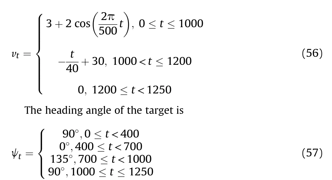
From the viewpoint of the adaptive control,Eq.s(1)and(3)are the optimal output. The reference model is

where the subscript m stands for the model.With the movement of the target, an error is introduced into the relative relationship by the target.The actual output is
For the convenience of calculation, we will treat the error as a vector. The generalized error vector is

4.2. The condition
The speed and direction of the target movement are unknown.Since the monitoring distance from the UAV to the target is given by a range,but not a specified value,it is not necessary to modify the center of the circular path in real-time. A new circular path is calculated when the distance error between the UAV and the target is accumulated to a certain extent.
With the movement of the target,in order to ensure monitoring effectiveness, it is necessary to timely decide the position of the circle center.As shown in Fig.4,before T1,the target is at the initial point and then starts to leave the initial point.
When circling in a coordinated turning mode, the body of the UAV is tilted and the flight attitude needs to be adjusted. Moving from a circling state to a horizontal flight state is a process with a minimum time that depends on the UAV’s physical parameters.This means that the UAV’s waypoints switching from a circular path to a new circular path are determined without changing the circling direction(clockwise or counterclockwise).We need to determine if the UAV has reached the switching point. The flight speed and altitude of the UAV used in this paper are constants. Therefore, on the circular path,the position of the UAV on the circular path can be decided by the heading angle.We use the direction of the target as the heading for the horizontal flight of the transition path.
The angle ψtbetween the direction of the target and the north is:

Fig. 4. Relationship between the UAV and the moving target.
where X(·)and Y(·)represent the abscissa and the ordinate of the variable in parentheses,respectively.That is,the heading angle for the horizontal flight is ψt(k). The heading angle ψswof the UAV at switch point is

where parameter ψcis the angle at which the UAV can change from a circle flight state to a horizontal one and its calculation is presented in next section.
When the heading angle ψt(k) of the UAV is the same as the switch heading angle ψsw(k), the system needs to determine whether it needs to plan the path or not.It is reasonable to predict future movements according to previous movements of the target.It is required that the target at the current trend of movement should not move out of the monitoring range when the UAV begins circling in another cycle. The UAV’s period for a circle is

As shown in Fig. 4, in ΔT1TkTk-1, the target’s movement length in one sampling period is

where el(k)means the magnitude of the vectorand eθ(k)is the angle between the vector e→(k)and the north.The distance traveled by the target during a cycle of the UAV Lcis

where dtis the sampling time. Note that Lkin Eq. (14) is actually equivalent to the estimated speed of the target. If the maximum speed of the target is known in advance, Lpshould be replaced by the maximum speed.
In the triangle formed by three points:the position of the UAV,the target position at time Tk, and the target predicted position at time Tcir,the predicted distance lpreduring this period can be found
by

By solving this equation and substituting Eqs.(13)and(14),we have

If the predicted distance does not satisfy the mission requirement, i.e., lpre<Dminor lpre>CDmax(C is a design parameter), a new circle center position is calculated.
4.3. The circular path algorithm
The new circle center is calculated in this subsection. Any prediction is adventurous for the target’s movement, and thus the calculation of a new circular path should depend on the target’s current position only. The varying rate of the center coordinate of the circle path is

Remarkably,Eq.(17)is the varying rate in a regular iteration.For initial or other special cases, we need to determine the absolute position of the center based on the position of the target relative to the UAV. Since the target may move in any direction, the UAV cannot circle on a fixed side(such as always on the west side of the target), but on a fixed side of the target’s direction of motion.
In Fig.5,according to the requirement,the distance D between the target and the circular path center can be


Fig. 5. Relationship between the current circular path and the target.
If the target remains stationary at the current position, the distance between the target and the UAV will be greater than the minimum distance Dminand shorter than the maximum distance Dmax. There is a constraint for the mission:

As shown in Fig.5,the center coordinate of the new circular path at this time is

where Ptis the target position at the same moment,i.e.,

where Puavis the position of the UAV at the same moment. It is worth noting that this coordinate does not need to be a global earth coordinate.
We can see that if the above conditions are satisfied,a new circle center is generated and given to the transition path planning algorithm. At this moment, if the reference model continues to be calculated in increment, an error will occur since the center of the circle has changed.At this point,the center coordinate needs to be updated.The complete calculation formula for the variables of the reference model should be
5. Transition path algorithm
The goal of this section is to develop a flyable path planning algorithm from the current circular path to a new circular path. In order to simplify the control model to focus on the tracking problem, the premise of the discussion here is to treat the UAV and target as research objects. Inspired by methods introduced in Ref.[2],we study only the path of the UAV without going deep into the dynamics. Therefore, on the point of the path planning, it is reasonable that three first-order models proposed in Ref. [28] are used to model the UAV.The UAV control channels include velocity,heading, and altitude. We assume that the UAV flies at a constant velocity over a constant altitude. Moreover, some popular general purpose flight controllers have the ability to control other channels and follow an expected input,such as constant velocity or constant altitude. Thus, for brevity, the heading angle ψ is the only variable that is designed. The model’s transfer function of the heading channel is

where μ >0 is the heading channel gain, and ψac(s) is the angle that needs to be changed. When the UAV needs to make a turn, a step response is put on the transfer as an input.The step response of the transfer function is

We organize the above descriptions into a pseudo-code form as follows.


Algorithm 1: Circular Path Calculating Input: the range l and the bearing angle θ Output: the coordinate of the center O 1 Initialization: R, D, Dmin, Dmax, v, dt, and C;2 Calculate the initial coordinate of the center O according to Eq. (20);3 Calculate the switch point ψsw(k) according to Eqs. (9)-(11);if ψ = =ψsw(k):5 4 Calculate the predict range lpre according to Eq. (16);6 if Dmin <lpre <CDmax:7 ˙O = 0; lm(k)8!!!θm(k)= lm(k-1)θm(k-1)+ ˙lm˙θm dt;else 10 ˙O = e→(k); lm(k)θm(k)9 11!!= lp(k)θp(k);12 endif 13 else 14 ˙O = 0;15 lm(k)θm(k)!!!dt;16 endif 17 O(k + 1) = O(k)+ ˙O·dt;= lm(k-1)θm(k-1)+ ˙lm˙θm

Fig. 6. Diagram for the current circular and new paths.
where ψc,as before,is the change angle.Taking the inverse Laplace transform of Equation (24), we obtain

The characteristic of the step input implies that the heading is a constant after turning the changed angle ψc. Eq. (25) matches segment AB.
Since it is a transition from a circular path to another one, as shown in Fig. 6, the entire transition (ABCD) can be viewed as a symmetrical process, i.e., the transition curve is symmetrical, and the axis of the symmetry is the perpendicular bisector of the line between centers O1and O2. Thus,one only needs to plan the path that flies out of the circle until the UAV’s heading is parallel to the line between these two circles, which is segment AB. On segment BC,the flight controller can fine-tune the heading angle of the UAV.If segment AB is calculated, we can symmetrize it to find segment CD.
5.1. The path planning for segment AB
Assume that the heading angle of the start point is ψs, and the heading angle of the end is ψe. The difference is

Now,considering the start and the end and substituting Eq.(25),the heading angle at time t is
Eq.(27)states that ψ(0)=ψsif t =0,and ψ(+∞)=ψeif t→+∞.In practice,it is not achievable and unnecessary for t to tend to be infinite. It is acceptable that the error is within 5% of the final value, which is three times the time constant, because of the straight-line segment BC.
To facilitate the computation,Eqs.(23)-(27)are deduced in the coordinate system shown in Fig. 6, and the actual path is then obtained according to the real situation.Substituting ψe=π/2 into Eq. (27), we obtain

The coordinate change of the UAV for the x-axis and y-axis is

Taking their derivatives and calculating the curvature,we have

If t = 0, κ0= μψc/|v|, then κab= κ0e-μt. It states that the curvature is continuous and monotonically decreasing for t∈[0, 3T].Thus,the curvature of segment AB is continuous and bounded.The upper bound is κ0, and the lower bound is zero.
5.2. The path planning for segment CD
We symmetrize the waypoints to generate segment CD.Although the waypoint is symmetrical about x=h, the velocity vector corresponding to the waypoint is symmetrical about the horizontal line, as shown in Fig. 7.
If t1(0 ≤t1≤3T) represents the time of a certain waypoint in segment AB, ψ(t1) represents the heading angle at t1. t2(0 ≤t2≤3T)is the time instance of the corresponding waypoint in segment CD, and ψ(t2) represents the heading angle at t2. Ttransis used to indicate the time of segment AB, i.e., 3T. The previous rule for determining the heading angle of segment CD can be expressed as

Substituting ψ(t) into Eq. (28) and solving Eq. (31), we have

As with the calculation process of segment AB,we can generate the curvature of segment CD by

If t=0, κcdwill be. Ttranshere is equal to 3T, which should be taken as+∞.Thus,theoretically,the curvature is 0 when t2= 0. There is a negligible heading angle error here, just like the end of segment AB.If t→+∞,or t is equal to Ttrans,κcdwill be
This means that segment CD is the same as segment AB in reverse order.

Fig. 7. Relationship between segments AB and CD.
5.3. Transition path algorithm
From Eqs.(30)and(33),we know that the curvature at the start of segment AB and the end of segment CD must be the same as the curvature of the circular path. The circle radius is

Substituting into the radius formula of a UAV circling over a point in a coordinated turn [29], we have

where g is the gravity acceleration, and Φmaxis the maximum roll angle of UAV.That is to say,under the constraint of the continuous curvature,the changed angle ψcis constant for a UAV.
Hence, the coordinate Pl(t) of segment AB at time t in the transition is obtained as

The coordinate Pl(t) starts at the origin of the local coordinate.That is, if t = 0, we have

It is noteworthy that all waypoints are computed in the Cartesian coordinate system xlOlylshown in Fig. 7, and the actual waypoints are required to rotate and move according to the position and distance of the two center points.
The global coordinate OgXgYgis set at the point where the target first appears with the x-axis pointing east and the y-axis pointing north, as shown in Fig. 8. The rotation angle η from the local coordinate to the global is

where x1and y1are the coordinate of the circular center O1,and x2and y2are the coordinate of the circular center O2. The rotation matrix is

with the coordinate set Plof the transition process relative to the local coordinate system, the coordinate set {Pg} in the global coordinate system can be obtained as

Fig. 8. Global and local coordinate.

where O’lis the coordinate of the origin Olof the local coordinate system in the global coordinate system OgXgYg, which can be generated by the coordinate of the center O1in the global coordinate system OgXgYg. We have

6. The worst case analysis and scope of the application
6.1. The shortest distance analysis
There is a shortest horizontal distance caused by the transition path planning algorithm. According to the principle of the special case in Section 4,we assume that the UAV can always move on the left side of the target according to Eq. (20).
For the convenience of analysis, in Fig. 9, we establish a Cartesian coordinate system with the first circling center as the origin,and x-axis points to the second center of the circle.According to the principle of the circular path algorithm, we have

where tyis the time at which the target starts to move from the yaxis when the UAV reaches the switching points. tciris the time cycle of one circle for the UAV. The shortest distance can be obtained by satisfying the minimum tyof Eq. (43). Substituting Eq.(12), we have

The minimum distance between two circular paths is dymin=vttymin. By taking the integral of Eq. (29) and using the Taylor formula, the horizontal shift xtrof the transition segment can be obtained as

A constraint is generated:

Accordingly, we have:

Fig. 9. Minimum distance between two circles.
where Dmax=mR,Dmin=nR,and v =kvt(m,n,k ∈R+).Considering the constraint represented by Eq. (19), we have

The complete constraints are
where K is a constant that depends on the physical constraint of the UAV, and M is a constant that depends on the video system.Whether the algorithm can run successfully depends on the selected UAV and mission needs.
Take the Aerosonde UAV in Ref.[30]’s Appendix E as an example.The speed of UAV is 10 m/s, and the minimum radius is 50 m. We assume that the speed of the target is 3 m/s.The requirement is that the maximum and minimum distances Dmaxand Dminare 500 m and 100 m, respectively. The left side of the inequality is 7.44, and the right side is 5.68. The horizontal distance in the transitional segment is 192.15 m, the shortest time is tymin= 110.91 s, and the shortest distance between the centers is vttymin=332.72 m.That is to say,between the two transitions,there is at least 48.42 m for the rudder to correct the heading. The constraints in Eq. (48) are thus met.
6.2. The longest distance analysis
According to the generation rule of the new circular path, as shown in Fig.10,we know that when the distance from the target to the switching point is the maximum monitoring distance Dmaxand the UAV has just passed the switching point,the distance between the two centers is maximum.The maximum distance between the current circular path center and the new one is

After the UAV enters the transition section,∠UU’O’is always an obtuse angle, which means that edge UO’ is the longest side of ΔUU’O’. The following equation is always true:
Fig.10. Maximum distance between two circles.

In Fig.10, it can be seen that the upper bound of the distance from the UAV to the new circular path is
Therefore, the distance from the UAV to the target cannot be greater than UO’+Dmin+ΔD,where ΔD is the distance traveled by the target.
Due to the unpredictability of the target movements,we assume that the target knows the motion of the UAV. We then design an escape path to consider the worst case. The worst case analysis is used to determine the design parameter C. In the worst case, the target moves along the line between the UAV and the target in a direction away from the UAV at all time.
When calculating the minimum distance, we know that, if the target stays in a critical state, the range l will not exceed the task requirements.If the target waits for the UAV to pass the switching point and then moves, the maximum critical monitoring distance will be reached when the UAV reaches the switching point next time. At this time, since there is an obtuse angle between the heading of the UAV and LOS,the movement of the UAV will result in an increase in distance. Since the UAV converges to a path that satisfies the monitoring range at a speed that is faster than the speed of the target,the relative distance will first increase and then decrease due to the movement of the UAV.
The maximum distance occurs when the tangent component of the UAV’s velocity vector is equal to the target’s vector,and we have

As a reminder,vutis the component of the UAV velocity vector in the tangential direction of the LOS.Substituting and simplifying Eq.(1), we have

Here,k is the ratio between the UAV’s speed and the target’s in Eq.(48).θ and ψ are the bearing angle and the heading angle of the UAV in Fig.2,respectively.Fig.11 portrays the relationship between the ratio k and the difference θ-ψ. When the speed gap between the UAV and the target is narrow,that is k→1,the heading angle ψ of the UAV equals to the beading angle θ.When the gap is vast,that is k→+∞,the heading of the UAV is perpendicular to the velocity of the target.

Fig.11. Relationship between the velocity ratio k and the difference θ- ψ.
In Fig.10, the tangential component of the velocity on the LOS will cause a change in θ:

The normal component on the line will cause the distance between the UAV and the target to change:

To obtain the maximum distance between the UAV and the target in process,it is necessary to solve Eqs.(54)and(55)under Eq.(53).Since Eqs.(54)and(55)are coupled,it is difficult to provide an analytical solution.
However, the change rate of the heading angle is exponential,and ratio k is always greater than 1. This means that the critical situation of Eq. (53) occurs at a point that is near to the starting point of segment AB. No matter how the target maneuvers, its range of motion is quite different from the upper bound of the surveillance range. Therefore, constant C is generally between 0.8 and 1. To a certain extent, reducing the threshold can compensate for the error that is caused by the fact that the target may be out of surveillance in extreme cases.
To obtain the maximum relative distance, it is easy to fall into the trap of local optimum by directly considering the direction of the target’s movement. To avoid this, we directly simulate the maximum distance at each moment when the UAV follows the transition path. We assume that the target always knows the movements of the UAV,and the longest distance between the UAV and the target at a certain moment definitely occurs when the target moves in the direction of the LOS at all time.In this way,the maximum distance between the UAV and the target at each moment is simulated.The target is to stand still for a control cycle when the UAV is about to reach the switching point and wait for the UAV to pass the switching point.
The simulation conditions are stated as follows. The speed of UAV is 10 m/s,and the minimum radius is 50 m.We assume that the speed of target is 3 m/s.At the beginning,the target is at the origin,and the UAV is located 100 m north of the target. After the UAV begins to circle, the target begins to move.When the UAV reaches the switching point,the target stops,waits for the UAV to pass the switching point,and continues to move forward,such that the UAV can circle more than once.

Fig.12. Influence of different C values on path planning.
Fig.13. Influence of different C values on the distance between the UAV and the target.
As shown in Figs. 12-14, the different line types indicate the different values of parameter C.There are five values for C:0.8,0.9,1, 1.1, and 1.2. The red line represents the UAV, and the blue one stands for the target.Fig.12 is a path diagram of the whole process of the UAV and the target.It can be seen that reducing the threshold causes the UAV to plan a new circular path in advance and vice versa. It is noteworthy that some lines for different C values coincide with each other,such as 0.8 and 0.9,1 and 1.1.The reason is that the new circle is not generated if the target moves in a small range.This repeated phenomenon in the next two figures verifies the robustness.Fig.13 is a plot of the distance between the UAV and the target in the whole process.It can be clearly seen from the change in distance that a short period of the transition process will exceed the expected monitoring range, but the reduction of the threshold compensates for this.
Suppose that the target knows the planning algorithm of the UAV at every moment.At any moment,the target moves toward the normal direction of the UAV at this moment from the beginning.
We can obtain a virtual maximum distance plot at each moment.The result is shown in Fig.14.An appropriate threshold can improve tracking performance.It should be noted that choosing a too small threshold will cause the entire algorithm to fail.
7. Simulation, comparison and discussion
7.1. Simulation background
To validate the proposed algorithm,simulations are conducted.First, we clarify the simulation background. Suppose that a UAV with a speed of 10 m/s and a minimum turning radius of 50 m is considered.The maximum speed for the ground target is 5 m/s.The movement of the ground target is arbitrary. The mission requirements are to keep the distance between the UAV and the target at least 100 m and no more than 500 m. These values are determined by the actual mission requirements and ratios that are between the speed of the UAV in the actual mission and the speed of the UAV used here.
The UAV is initially at(0 m,100 m),heading to the east at a fixed speed of 10 m/s.The target is placed at the origin.The speed of the target changes over time as shown in the motion equation below:
The speed and the heading angle are presented in Fig.15.
7.2. Simulation

Fig.15. Speed and the heading angle of the target.

Fig.16. Path for the UAV and the target.

Fig.17. Curvature curve over the entire simulation.
Fig.18. Heading angle for the entire path.

Fig. 20. Distance curve between the UAV and the target.
First,the path planning algorithm plans the UAV path according to the target path. Fig.16 shows the planned path of the UAV and the target.The target path is a polyline.The blue dotted line is the target trajectory.The red solid line is the UAV path.The black solid line is the line between the UAV and the target, which is drawn every 50 s to mark the time. Fig. 17 shows the curvature of the whole path. The curvature is continuous for the whole simulation time just like the analysis in Section 5. Fig.18 depicts the heading angle curve for the whole path.To present the continuous heading angle,the sine value of the heading angle is plotted in Fig.19.Fig.20 portrays the distance between the UAV and the target.Although the distance line fluctuates at all times, the range l is larger than the minimum distance Dminand smaller than the maximum distance Dmax. This means that the tracking task is completed.
7.3. Comparison and discussion
As can be seen in Fig.16,the UAV is always on the left side of the target, as are the laser spots. The UAV does not pass above the target. We compare the algorithm in Park et al. [26] and perform the simulation under the exact same conditions.

Fig. 21. Planning path of the algorithm in Ref. [26].

Fig. 22. Comparison of observation angles between Park’s algorithm and our algorithm.
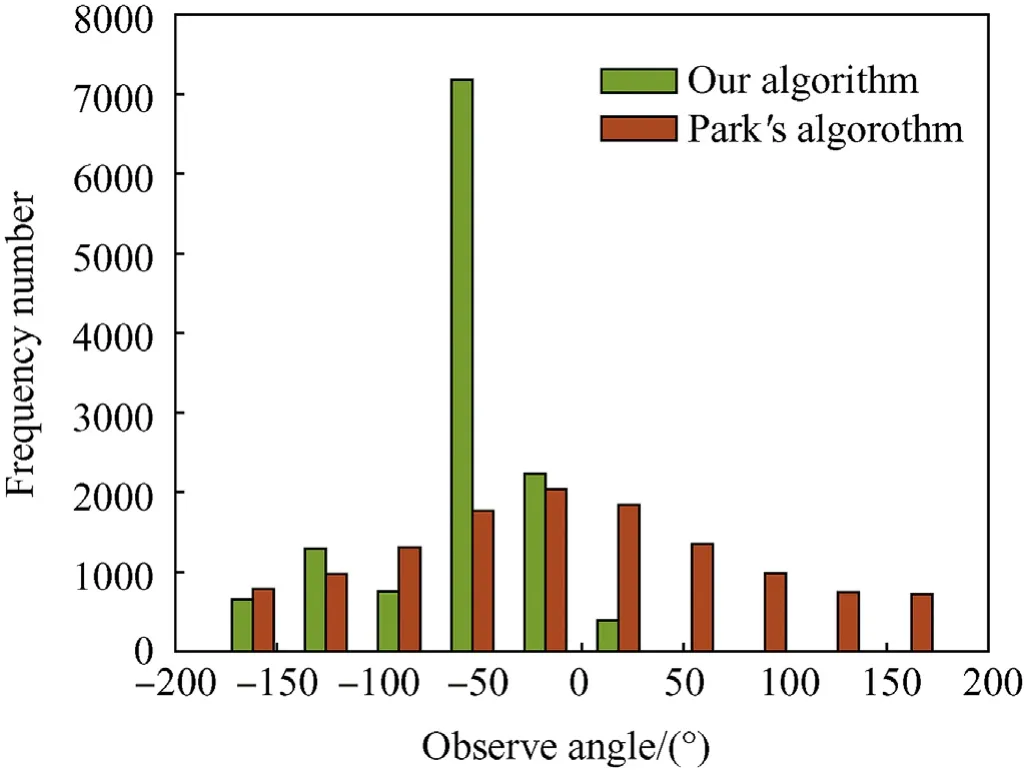
Fig.23. Histogram for comparison of observation angles between Park’s algorithm and our algorithm.
The path of the UAV and the target is shown in Fig.21.The timevariant target makes the UAV in Ref.[26]busy.Like most algorithms that take the target as the center point of the circle, the UAV appears on different sides of the target at different times.
In order to compare the monitoring angle,the observation angle θobbetween the LOS and the normal direction of the target’s velocity is plotted. As can be clearly seen in Figs. 21 and 22, the bearing angle of our algorithm is between 50 and-170°;using the conventional algorithm, the angle is distributed between -180°and 180°. Although the heading of the target is arbitrary, most of the observation angle is around -50°. As the UAV converges towards the circular path, the range of observation angles becomes increasingly small.From this,we can give the reliable area of laser.By combining with the azimuth and position of the UAV, we can calculate the region where the optimal laser reflection can be received. This means that the laser-designating task can be done better than other existing methods (see Fig. 23).solution, such as searching the optimal UAV speed for minimizing the cost, and having an adaptive parameter C for improving the tracking robustness;the other is about modeling the path planning problem for multiple UAVs to track and laser-designate an unknown target with more complicated motion and situations using Petri nets[32] [33]and look-ahead methods [31].
Acknowledgments
The authors extend their appreciation to the Deanship of Scientific Research at King Saud University for funding this work through research group number (RG-1440-048).
Appendix A
This appendix is a list of notations used in the paper.

Table 1 Notation list.
8. Conclusions
This work studies path planning whereby a target is tracked and laser-designated by a UAV. For constraining the bearing angle, we propose a new way of tracking.The circular path is on the same side of the target at all the time.The calculation method of the circular path center is given.We propose a circular path planning algorithm for calculating the circular path location based on the UAV-target range and the bearing angle in real time. We also develop a transition path planning algorithm for transitions between circular path, and this algorithm considers the minimum turning radius of the UAV. The mission is divided into two parts based on the two algorithms. The circular path planning algorithm completes the monitoring location design for different target locations, and the transition path planning algorithm completes the transition between different circular paths. The effectiveness and reliability of the methods are demonstrated by an analysis of upper and lower bounds. A restriction condition is given for the UAV and the requirement. A series of simulation examples are presented to verify the proposed method. Compared with the traditional methods, we can see that the proposed method is more efficient when a UAV laser-designates a target. Future work will mainly include two aspects:one is about the improvement of the technical
- Defence Technology的其它文章
- Analysis of sliding electric contact characteristics in augmented railgun based on the combination of contact resistance and sliding friction coefficient
- Aerodynamics analysis of a hypersonic electromagnetic gun launched projectile
- Synergistic effect of hybrid Himalayan Nettle/Bauhinia-vahlii fibers on physico-mechanical and sliding wear properties of epoxy composites
- Study on dynamic response of multi-degree-of-freedom explosion vessel system under impact load
- An investigation on anti-impact and penetration performance of basalt fiber composites with different weave and lay-up modes
- Modeling and simulation of muzzle flow field of railgun with metal vapor and arc