基于对偶理论的椭圆变分不等式的后验误差分析(英)

a(u,v −u)≥ℓ(v −u), ∀v ∈K,

E(v)=J(v,Λv)=F(v)+G(Λv), ∀v ∈V,

J∗(Λ∗q∗,−q∗)=F∗(Λ∗q∗)+G∗(−q∗).

1 Introduction

For practical applicaton of algorithms, one of the most important points is the assessment of the reliability of numerical solutions. This reliability hinges on our ability to estimate errors after the solution is computed, such an error analysis is called a posteriori error analysis. A posteriori error estimates provide quantitative information on the accuracy of the solution and are the basis for the development of automatic,adaptive algorithms in engineering applications. In a typical a posteriori error analysis,after a numerical solution is found, the solution is used to compute an error estimator. However, a posteriori error estimation for partial diあerential equations received attention more than three decades ago[1-5]. Nowadays the literature on this subject is vast, see [6-10] and the references therein. Most error estimators can be collected into three main groups: the residual type, the gradient recovery type and the equilibrate data type. Various residual quantities[2,3,6,10,11]are used to capture lost information going from accurate solution to numerical solution,such as the residual of the equation,boundary condition, the residual from derivative discontinuity, the residual of material constitutive laws, and so on. The type based on gradient recovery[12-14]is based on averaging (smoothing) approximate solutions obtained by the finite method. These types of post-processing procedures give new approximations, which often are much more accurate. For this reason, the diあerence between the direct approximation and the averaged one can be used as an error estimator. Complementary energy principles were applied for getting error estimates in[15-18]and in other papers. They formed the basis of equilibrated data type which apply special numerical procedures designed for getting the so-called “equilibrated function” in complementary energy principles. Two desirable properties of an a posteriori error estimator are the reliability and eきciency.The reliability requires the actual error to be bounded by a constant multiple of the error estimator,up to perhaps a higher order term,so that the error estimator provides a reliable error bound. The eきciency requires the error estimator to be bounded by a constant multiple of the actual error, again perhaps up to a higher order term, so that the actual error is not over-estimated by the error estimator. The study and applications of a posteriori error analysis is currently an active research area, and the related publications grow fast.

Most of the work on a posteriori error analysis has been devoted to ordinary boundary value problems of partial diあerential equations. In applications,an important family of nonlinear boundary value and initial-boundary value problems is that associated with variational inequalities. Although several standard techniques have been developed to derive and analyze a posteriori error estimates for finite element solutions to problems in the form of variational equations, they do not work directly for a posteriori error analysis of numerical solutions to variational inequalities. Particularly, the inequality aries as a result of the presence of a non-diあerentiable functional. Many works deal extensively also with a priori estimates,but residual type error estimators were studied for an elliptic variational inequality of the second kind in [19,20]. However, a major diきculty in solving the variational inequality of the second kind numerically is the treatment of the non-diあerentiable term. In practice, there are several approaches to circumvent the diきculty. One approach is to introduce a Lagrange multiplier for the non-diあerentiable term, or by an iterative procedure or the regularization method.

In this paper, we mainly consider the situation where the function J is of a separated form, J(v,Λv) = F(v)+G(Λv), ∀v ∈V, we make use of a diあerent bounded operator form Λv and functional form F, G to formulate their dual problems for a friction contact problem and an obstacle problem. we give a posteriori error analysis via duality theory by the regularization method for elliptic variational inequalities[21]. The idea of the regularization method is to approximate the non-diあerentiable term by a sequence of diあerentiable ones. An approximating diあerentiable sequence in the regularization method depends on a small parameter ε ≥0. The convergence is obtained when ε goes to 0. but if ε is too small, the numerical solution of the regularized problem cannot be computed accurately. Thus, it is highly desirable to have a posteriori error estimates which can give us computable error bounds once we have solutions of regularized problems.

This paper is organized as follows. In section 2 and section 3, we, respectively,introduce a friction contact problem and an obstacle problem, give their regularized problems, variational inequalities. Choosing a diあerent bounded operator form and functional form, we formulate their dual problems for these models, on which our later a posteriori error analysis will be based. In section 4, we establish a general framework for a posteriori error estimates of an obstacle problem by using duality theory in convex analysis. The general a posteriori error estimate is featured by the presence of a dual variable. Diあerent a posteriori error estimates can be obtained with diあerent choices of the dual variable. At last, we make a particular choice of the dual variable that leads to a residual-based error estimate of the model problem and explore the eきciency of the error estimate.

2 A frictional contact problem and its regularized problem

Let Ω be a bounded domain in Rd(d ≥1),with a Lipschitz boundary Γ. Let Γ1⊂Γ be a relatively closed subset of Γ, and denote Γ2= ΓΓ1for the remaining part of the boundary. Since the boundary Γ is Lipschitz continuous, the unit outward normal vector n exists a.e.on Γ. We will use ∂/∂n to denote the outward normal diあerentiation operator, which exists a.e.on Γ. Assume f ∈L2(Ω) and g ＞0 are given.

Introducing the space V = H1Γ1(Ω) = {v ∈H1(Ω) : v = 0 a.e. on Γ1}, then a frictional contact problem is the following elliptic variational inequality of the second kind: find u ∈V such that

where

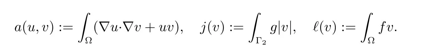
Here and below, to simplify the notation for an integral, we usually do not explicitly display the infinitesimal volume or surface or line element which can be easily identified by the domain where the integration is taken. The model we use is a so-called simplified friction problem[22]as it can be viewed as a simplified version of a frictional contact problem in linearized elasticity.

Since the bilinear form a(·,·) is continuous and V-elliptic, the functional j(·) is proper, convex and continuous, and the linear functional ℓ(·) is continuous. Moreover,since the bilinear form a(·,·) is symmetric, the variational inequality (1) is equivalent to the minimization problem: find u ∈V such that

where E is the energy functional

Existence and uniqueness of a solution for the problems (1) and (2)-(3) follow from a classical result[23]. Moreover, the equivalence between the variational inequality and the minimization energy functional problem can be established in a standard way.

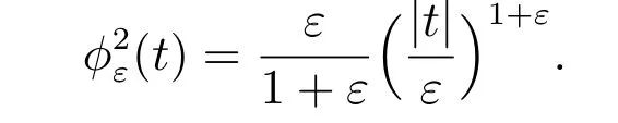
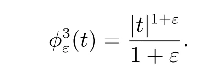
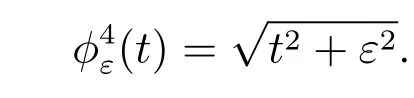
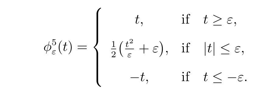
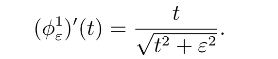
For a given non-diあerentiable term, there are many choices for a sequence of differentiable approximations. Let us list five natural choices of a regularizing sequence for the frictional problem (similar to the first two choices are taken from [24]).

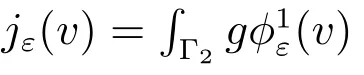
Choice 2jε(v)=∫Γ2g(v) with

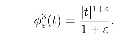
Choice 3jε(v)=∫Γ2g(v) with

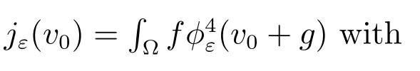
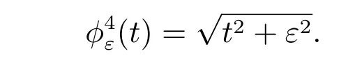
Choice 4jε(v)=∫Γ2g(v) with

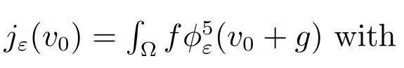
Choice 5jε(v)=∫Γ2g(v) with

2.1 Dual formulation

We derive a dual formulation for the problem (2)-(3), following the framework presented in [25]. Let V and Q be two normed spaces, V∗and Q∗denote their dual spaces. The duality pairings in both V,V∗and Q,Q∗will be denoted by〈·,·〉. Assume there exists a linear continuous operator Λ ∈L(V,Q). The transpose Λ∗∈L(Q∗,V∗)of the operator Λ is defined through the relation

Let J be a functional mapping V ×Q intoWe consider the minimization problem(the primal problem)

Its dual problem is defined as

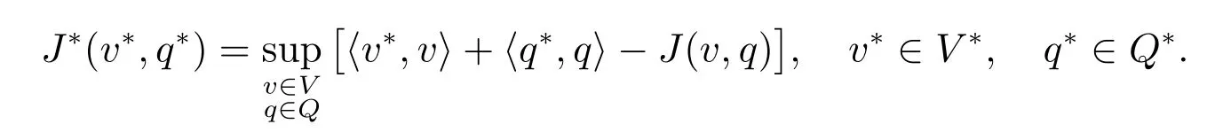
where J∗:Q∗×V∗→is the conjugate function of J:

Now for the minimization problem (2), let

we introduce the functional

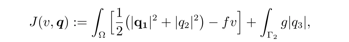
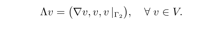
where q = (q1,q2,q3) ∈Q, and introduce a linear bounded operator V →Q by the relation

Obviously

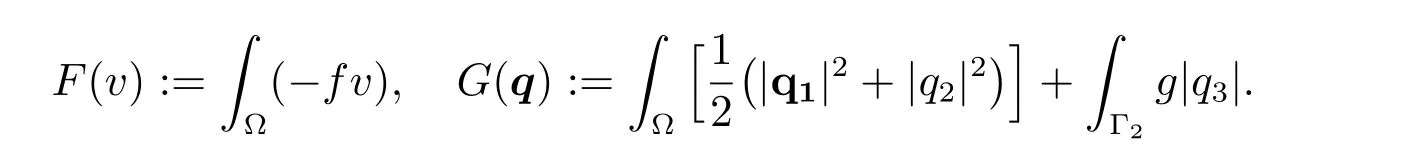
where

Then the minimization problem (2) can be rewritten as: find u ∈V such that

and the corresponding conjugate function J∗of the functional J:

We have

and

Define the set of admissible dual functions as

Then the conjugate function is

The dual problem of (5) can now be stated as: find p∗∈Q∗f,gsuch that

Note that the mapping q∗→J∗(Λ∗q∗,−q∗) is strictly convex over Q∗f,g. By the result in ([21], Theorem 2.39), the dual problem (6) has a unique solution p∗∈Q∗f,g, and

where u ∈V is the unique solution of the model problem.

2.2 A posteriori error estimates

As far as the practical computation is concerned, a convergence result and an a priori error estimate are not enough for a completely numerical analysis with the regularization method. A posteriori error estimates are more desirable that will provide a quantitative error bound once a solution of the regularized problem is an error bound.Here,for a frictional contact problem,we will use the duality theory to drive some other a posteriori error estimates, and then discuss the applications to the regularization method with various choices of the regularization sequence.

Since G(q) is not Gateaux diあerentiable, we consider the energy diあerence

Using (1) with v =uε, we find that

Therefore

On the other hand, applying Theorem 2.40 in [21], we have

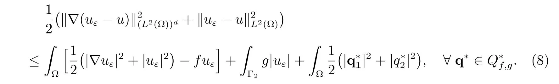
for any q∗∈Q. Hence, we have the general inequality for a posteriori error analysis

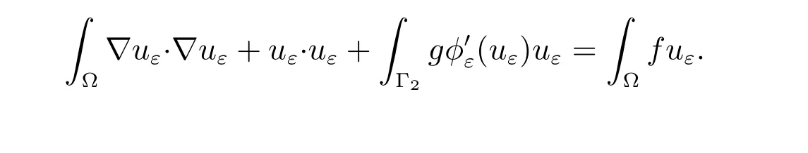
Since φεis diあerentiable, the variational inequality (4) is equivalent to the equality

Thus uεis the weak solution of the elliptic boundary value problem

From (9), we observe that if the regularizing function φ satisfies the inequality

then a natural selection of an auxiliary field q∗in the basic inequality (8) is

From (8), the following a posteriori error estimate is obtained

Taking v =uε∈V in (9), we find that

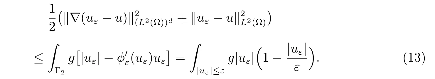
Therefore, we can write the a posteriori error estimate in the form of

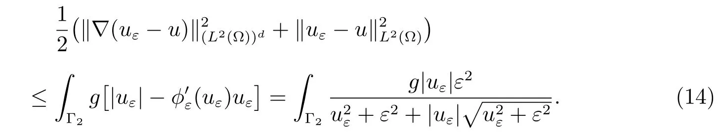
The regularizing functions in the Choices 1,4,and 5 satisfy the inequality(10). Hence,we have the following a posteriori error estimates.

For theChoice 1, we have

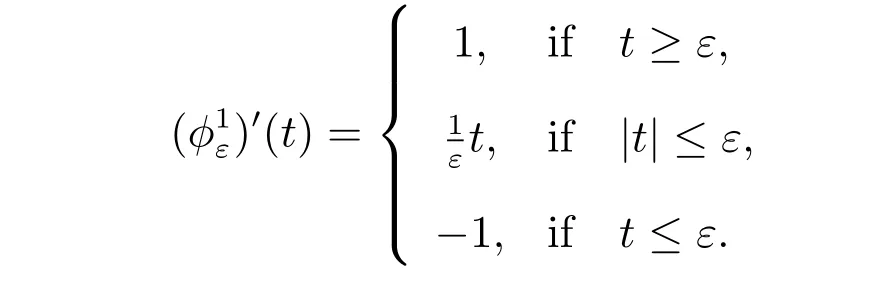
Thus the a posteriori error estimate is

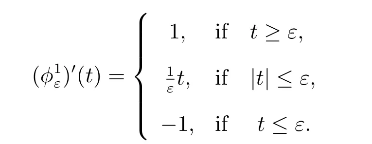
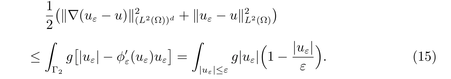
For theChoice 4, we have

Thus the a posteriori error estimate is

For theChoice 5, we have

Thus the a posteriori error estimate is

So we have the same form of a posteriori error estimate as that given in (13). For the Choices 2 and 3, the regularizing functions do not satisfy the inequality (10), but it is still possible to construct an admissible field q∗from uεto produce a good error bound.

3 An obstacle problem and its regularized problem

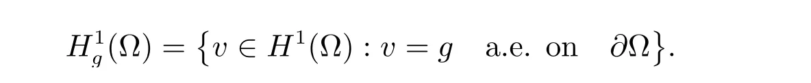
The model problem to be discussed is a generalized version of an obstacle problem considered in[26]. Let Ω ∈Rdbe a Lipschitz domain. In the study of obstacle problems for applications,d=2. However,all the arguments below are valid for any dimension d.Let f ∈L2(Ω)and g∈H1/2(∂Ω)be given non-negative functions. Denote the admissible set by

where

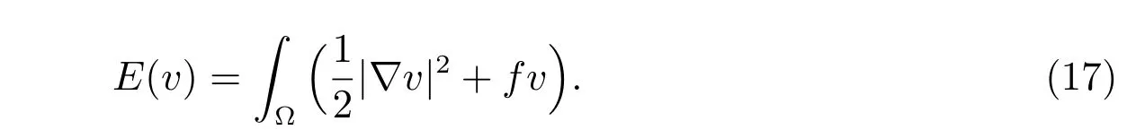
Then the obstacle problem is: find u ∈K such that

where

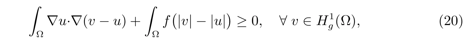
The problem(16)-(17)is equivalent to an elliptic variational inequality of the first kind:find u ∈K such that

a(u,v −u)≥ℓ(v −u), ∀v ∈K,

where

Existence of a unique solution of the problem follows from the standard result on the unique solvability of variational inequalities of the first kind ([21], Theorem 1.24)

To develop a regularization method, the obstacle problem (16)-(17) is also written as the problem: find u ∈(Ω) such that

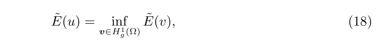
where

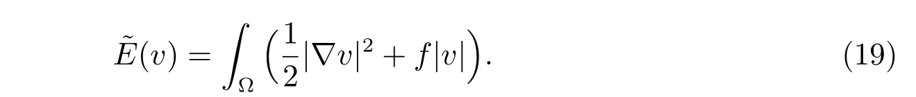
The problem (18)-(19) is equivalent to an elliptic variational inequality of the second kind: find u ∈(Ω) such that

where

Now,introducing v0=v−g for v ∈H1(Ω),then a solution of the problem(18)-(19)is u=u0+g and u0∈(Ω) such that

where

The problem (21) is equivalent to an elliptic variational inequality of the second kind:find u0∈(Ω) such that

where

Proposition 1 The problem(16)-(17)and the problem(18)-(19)are equivalent.

Proof First, the problem (18)-(19) and the variational inequality (22) have a unique solution([21], Theorem 1.25). Next, the equivalence proof between the problem(16)-(17) and the problem (18)-(19) ([21], page195, Theorem 5.1). Therein, applying some results from [21] as follows: if v ∈H1(Ω), then |v|∈H1(Ω) and

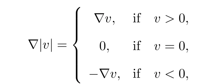
Combining with the uniqueness of a solution to the problem (18)-(19), we have u =|u| ≥0 in Ω. Hence, the solution to the problem (18)-(19) is also the unique solution of the problem (16)-(17).

The regularized problem is to find u0,ε∈(Ω) such that

or uε∈(Ω) such that

The relation between the solutions of the two problems is uε=u0,ε+g. We can prove that under conditions, u0,ε→u0(equivalently, uε→u) as ε →0 ([21], Lemma 5.2).

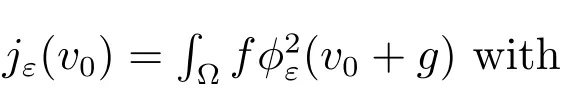
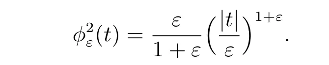
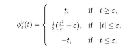
For a given non-diあerentiable term, there are many choices for a sequence of differentiable approximations. Let us list five natural choices of a regularizing sequence for the obstacle problem (the first two choices are taken from [26]).

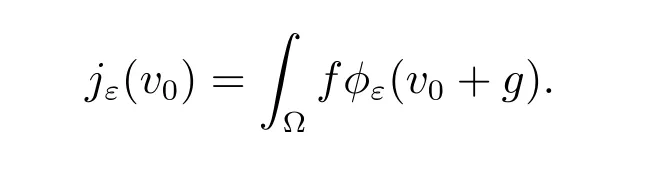
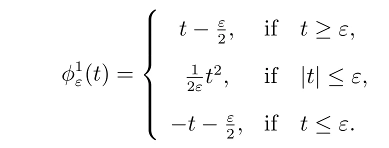
Choice 1jε(v0)=∫Ωf(v0+g) with

3.1 Dual formation

For the obstacle problem (18)-(19), we adopt the function spaces

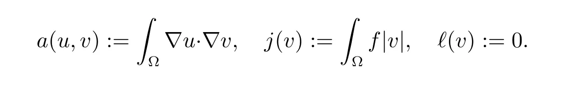
and the operator Λv =∇v, ∀v ∈V, and the functional

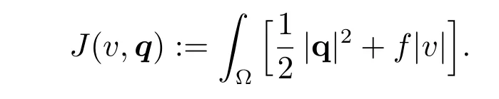
Then obviously

E(v)=J(v,Λv)=F(v)+G(Λv), ∀v ∈V,

where

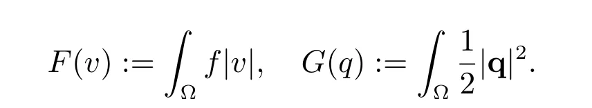
Therefore, the minimization problem (18)-(19) can be rewritten as: find u ∈V such that

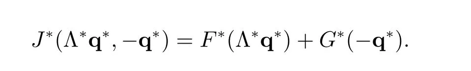
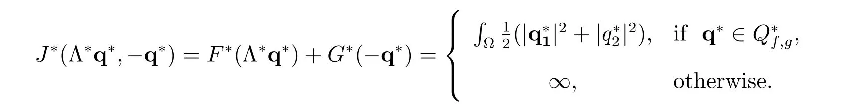
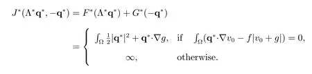
the corresponding conjugate function J∗of the functional J is

J∗(Λ∗q∗,−q∗)=F∗(Λ∗q∗)+G∗(−q∗).

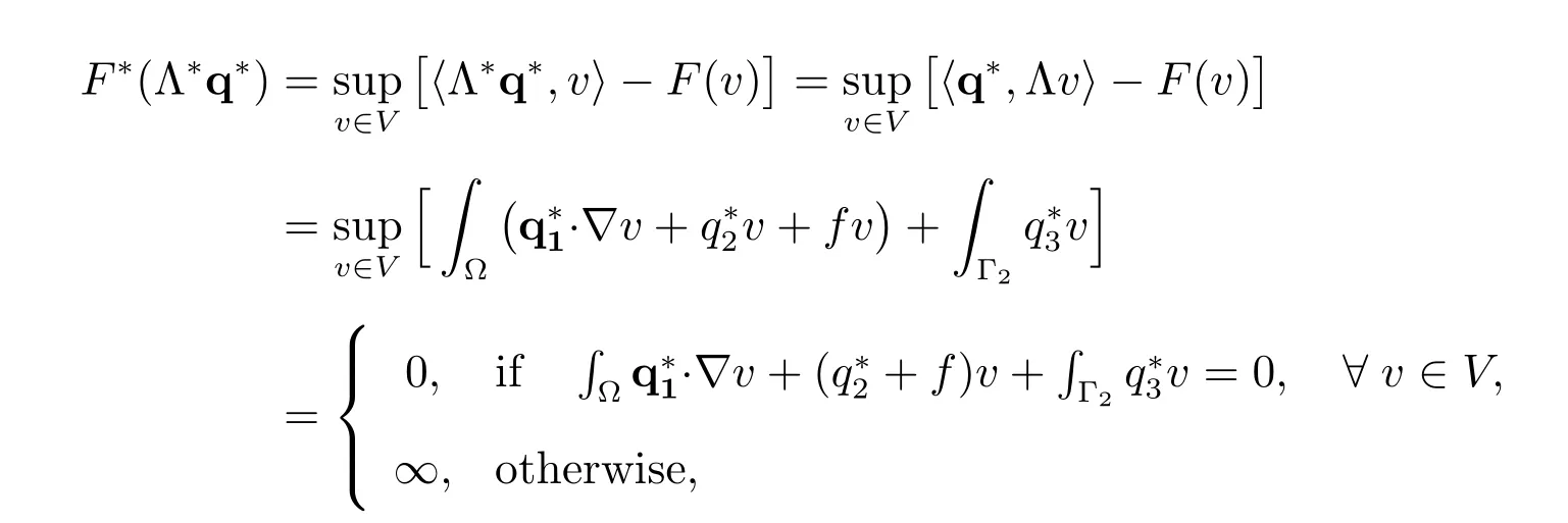
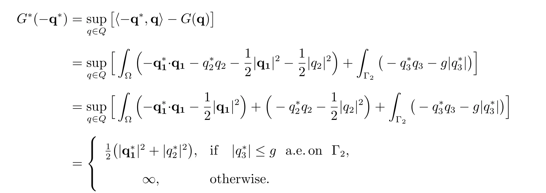
We have

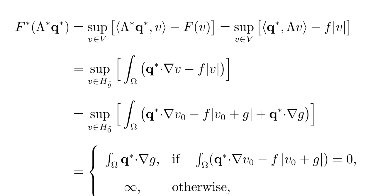
and

Define the set of admissible dual functions:

Then the conjugate function becomes

The dual problem of (25) can now be stated as: find p∗∈Q∗csuch that

Note that the mapping q∗→J∗(Λ∗q∗,−q∗) is strictly convex over. By Theorem 2.39 in [21], the dual problem (26) has a unique solution p∗∈, and

where u ∈V is the unique solution of the model problem.

3.2 A posteriori error estimates

Similarly,here,for an obstacle problem,we also use the duality theory to drive some new a posteriori error estimates,and then discuss the applications to the regularization method with various choices of the regularization sequence.

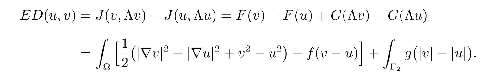
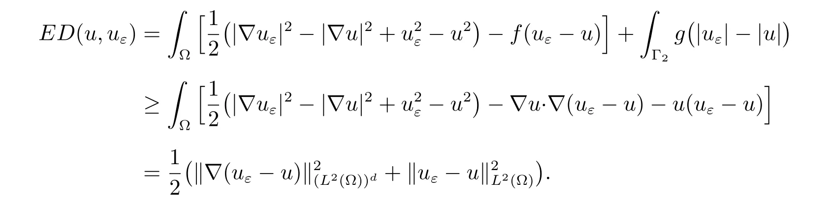
Since F(v) is not Gateaux diあerentiable, we consider the energy diあerence

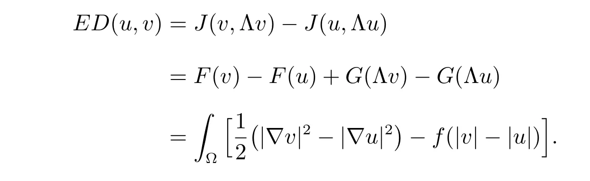
Using (20) with v =uε, we find that

Therefore

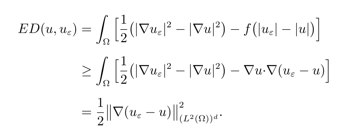
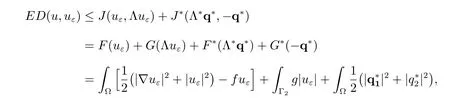
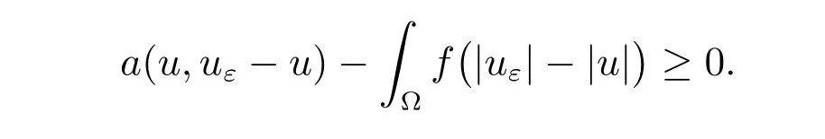
On the other hand, applying Theorem 2.40 in [21], we have

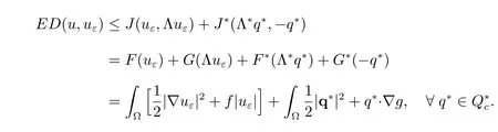
Hence, we have the general inequality for a posteriori error analysis:

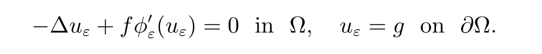
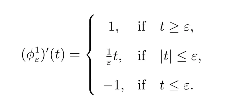
Since φεis diあerentiable, the variational inequality (24) is equivalent to the equality

Thus uεis the weak solution of the elliptic boundary value problem

From (29), we observe that if the regularizing function φ satisfies the inequality

then a natural selection of an auxiliary field q∗in the basic inequality (28) is

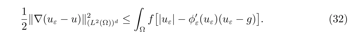
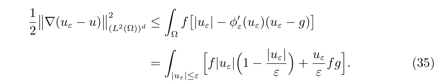
From (28), the following a posteriori error estimate is obtained

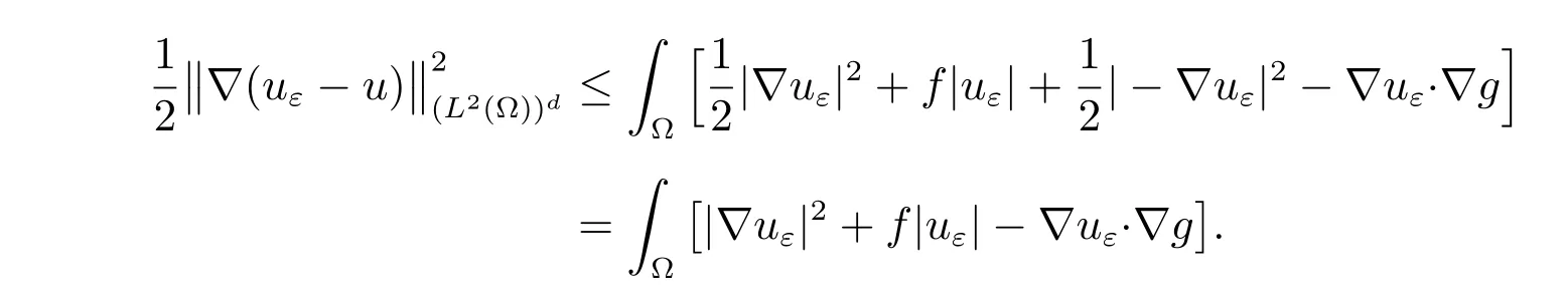
Taking v =uε−g ∈(Ω) in (29), we find that

Therefore, we can write the a posteriori error estimate in the form of

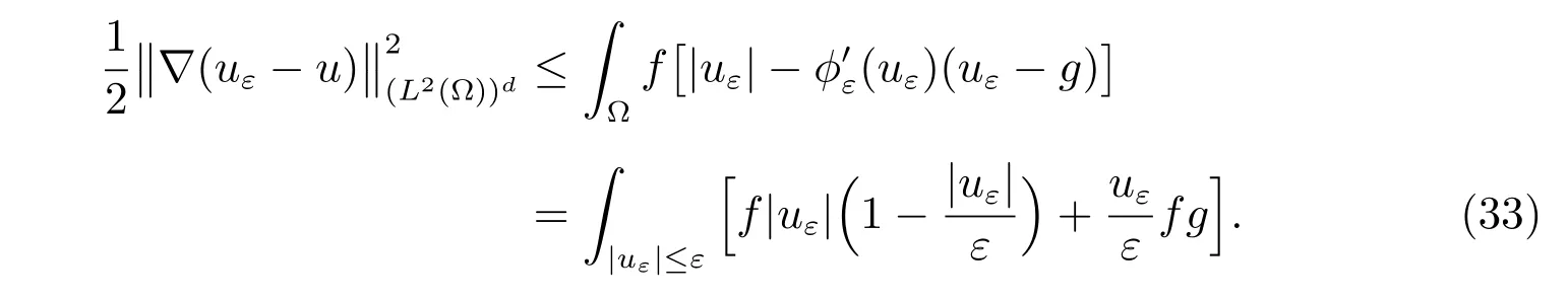
The regularizing functions in the Choices 1,4,and 5 satisfy the inequality(30). Hence,we have the following a posteriori error estimates.

For the Choice 1, we have

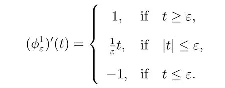
Thus the a posteriori error estimate is

For the Choice 4, we have

Thus the a posteriori error estimate is

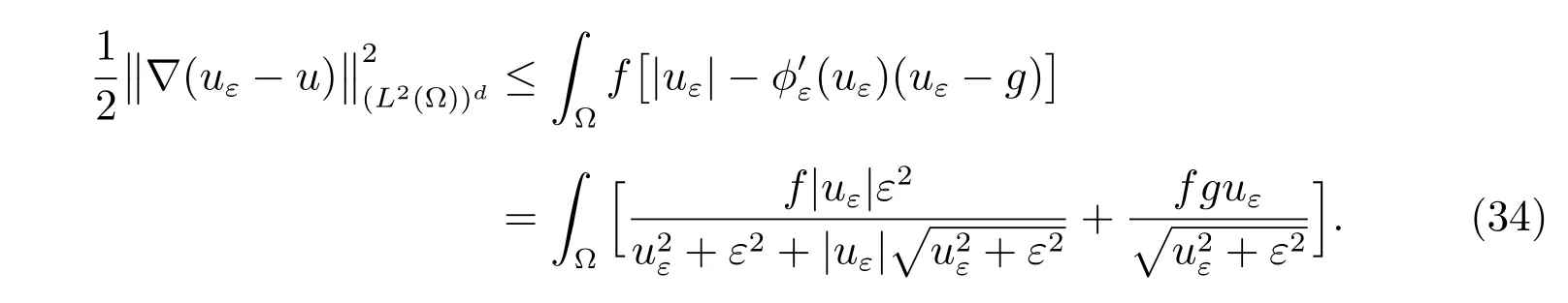
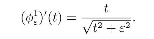
For the Choice 5, we have

Thus the a posteriori error estimate is

So we have the same form of a posteriori error estimate as that given in (33). For the Choices 2 and 3, the regularizing functions do not satisfy the inequality (30), but it is still possible to construct an admissible field q∗from uεto produce a good error bound.

4 A general framework for a posteriori estimates

In this section, let w be an arbitrary approximation of u ∈V, the unique solution of the frictional contact problem (1) or the obstacle problem (18), we present a general framework for a posteriori estimates of the error (u −w). The error bounds are computable from the known approximation w. For the frictional contact problem,a general framework has been given in [21] for a posteriori estimates of elliptic variational inequalities. In the following, for the obstacle problem, we deduce its general framework by use of a similar method. By using (19) and (20), we obtain

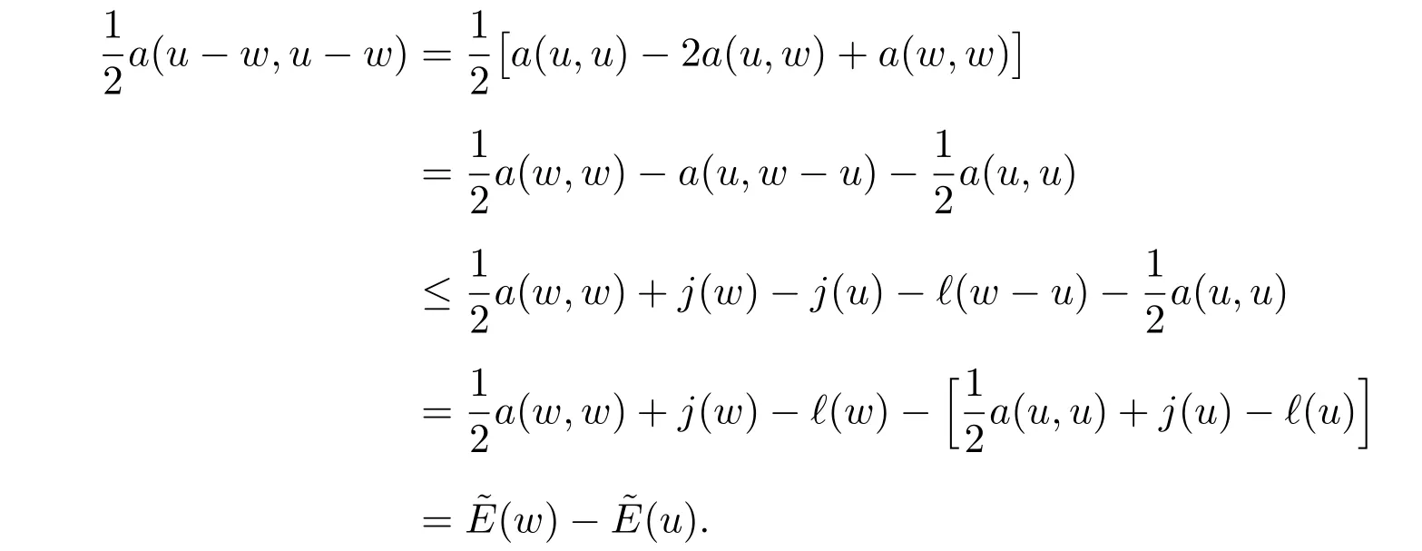
On the other hand, let p∗be the solution to the dual problem (26). Relation (27)implies

Therefore

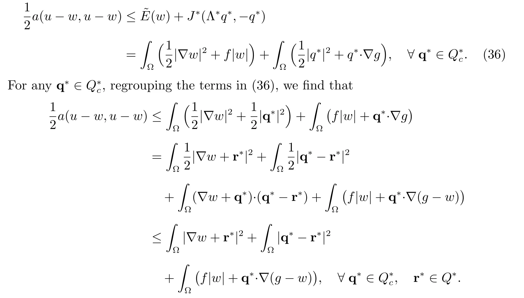
Thus, we have established the following result.

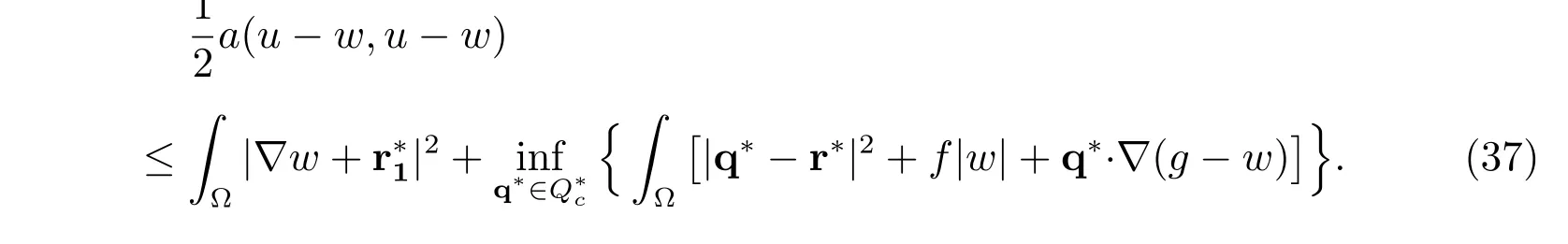
Theorem 1Let u ∈(Ω) be the unique solution of (20), and w ∈V an approximation of u. Then the following estimate holds for any r∗∈Q∗:

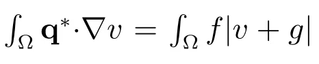
Let us now deal with the second term ∏on the right side of the estimate (37). First,from the definition of, it follows that

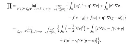
Define the residual

Then

Combined with Theorem 1, we can derive the following result.

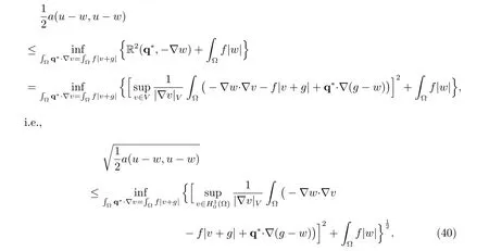
Theorem 2Let u ∈V be the unique solution of (20), and w ∈V an approximation of u. Then the following estimate holds for any r∗∈Q∗:

where the residual R(q∗,r∗) is defined by (38).

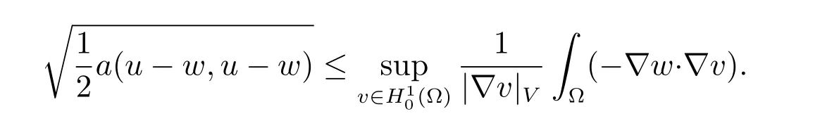
With the special selection r∗= −∇w, the error bound (39) leads to the following error estimate

In the limiting case f =0, the problem (20) reduces to the variational equation

We observe that correspondingly, the estimate (40) reduces to the familiar form

5 Conclusions

In this paper, we mainly make use of a diあerent bounded operator form Λv and functional form F, G to study a posteriori error analysis via duality theory for the regularization method for a frictional contact problem and an obstacle problem. We also establish a general framework to derive reliable residual type error estimators for the above obstacle problem by applying a posteriori error analysis via duality theory in convex analysis. Certainly, the same technique presented in this paper can be used to derive a posteriori error estimates for the regularization method for other variational inequality problems.