Modeling and analysis of car-following behavior considering backward-looking effect∗

Dongfang Ma(马东方), Yueyi Han(韩月一), Fengzhong Qu(瞿逢重), and Sheng Jin(金盛)

1Ocean College,Institute of Marine Information Science and Technology,Zhejiang University,Hangzhou 310058,China

2College of Civil Engineering and Architecture,Institute of Intelligent Transportation System,Zhejiang University,Hangzhou 310058,China

Keywords: traffic flow,car-following model,visual angle,backward-looking effect

1. Introduction

Car-following models have always been an important research topic in the field of microscopic traffic flow and statistical physics. It has significant application in complex systems,traffic simulation,and intelligent driving.Numerous carfollowing models have been developed in the past decades,and they have important theoretical significance for a profound understanding of complex random characteristics,critical phase transitions,and stability of traffic flow.

Since the concept of car-following model was proposed in the early 1950s,hundreds of important car-following models have been proposed.[1-8]In recent years, many different car-following models[9-18]are put forward under the modern traffic situation and lots of scholars devote themselves in investigating the behavior of car following.[19]To enrich the traffic flow theory, some scholars proposed extended traffic flow models.[20]However, most models only consider the driver’s perception of the leading vehicle’s motion status information and completely ignore the stimulation of rear vehicle’s motion.In an actual driving environment, the driver will also observe the movement of rear vehicle through the rearview mirror and use it as a basis for adjusting the speed of own vehicle to prevent the rear vehicle from rear-end collision due to its own emergency braking. Especially when traffic is congested or vehicles frequently change lanes,the rear-view effect is more obvious. At the same time, when the distance between two vehicles in the front and rear is small,a severe deceleration of the front vehicle may cause the rear vehicle to brake urgently or even cause a rear-end collision, which may cause congestion and security risks. Therefore, to ensure their own safety and smooth traffic,the drivers will comprehensively judge the state of leading and following vehicles to adjust their driving behavior when driving.The rear-view effect helps the driver to maintain the distance between front and rear vehicles as consistent as possible which effectively stabilizes the traffic flow.

In recent years,the effect of rear car’s movement on carfollowing behavior has been gradually considered, and relevant models have been established. Sun et al.[21]proposed a car-following model by considering the backward-looking effect and speed difference and showed that the consideration of above factors simultaneously can enhance the stability of traffic flow and effectively suppress the traffic jam. Ge et al.[22]proposed a feedback control car-following model that considers the headway of front and rear vehicles and conducted a stability analysis of the model from a cybernetic perspective, confirming the important role of feedback control signals in suppressing and alleviating traffic congestion. Chen et al.[23]proposed a car-following model that considers driver’s sensory memory and the backward-looking effect, exhibiting good traffic flow stabilization performance. Based on the GIPPS safety distance model, Yang et al.[24]further considered the backward-looking effect and developed a new model.They found that the consideration of backward-looking effect has three types of effects on traffic flow:stabilization,destabilization, and nonphysical phenomena. These models provide important reference value for understanding the effect of rear car on the car-following behavior and have important significance for understanding the factors influencing car-following behavior in a complex environment.

However,all the above-mentioned models assume that the drivers can accurately perceive the speed, distance, and other variables of the rear car, contrary to the driver’s perception characteristics.Related studies in the field of psychology[25,26]show that the driver cannot accurately perceive the state parameters such as speed and distance; therefore, the following car model based on accurate parameters cannot describe the real driving behavior well. In an actual driving environment,the driver mainly relies on visual information to perceive the vehicle’s movement and then changes his or her own acceleration. In recent years, studies have also been conducted on the visual angle car-following model.[27-30]Jin et al.[28]introduced visual angle as a stimulus for driver to perceive the leading vehicle and built a relevant car-following model. The simulation results show that the model can better describe the characteristics of driver’s asymmetry in acceleration and deceleration and speed fluctuation. Recently, Ma et al.[29]proposed that the solid angle composed of the width and height of the vehicle is a factor influencing the car-following behavior and established the new model using the solid angle as the influencing factor. However,all the car-following models based on visual information focus on the influence of leading vehicle. It is still theoretically significant how to reconstruct the car-following behavior under the combined influence of front and rear vehicles and define more reliable stability conditions of traffic flow parameters.

Based on the above analysis,this study assumes that during the car-following behavior,the driver judges the movement of leading car and following car depending on visual information and establishes the calculation method of visual angle and its rate of change of front and rear vehicles. On this basis,a fusion mechanism is proposed for the visual information of front and rear vehicles,and then a car-following model is developed under the influence of backward-looking effect. Further analysis of model characteristics and advantages such as stability analysis, numerical simulation, and model comparison provides a basis for building a more realistic and effective microscopic traffic flow model.Using visual angle as influencing factor is a better indicator of human drivers’ awareness.Especially for the rear car, the drivers are harder to perceive the headway and the velocity. The only way to judge the rear car’s behavior is observing the change of the rear car’s size in the driving mirror. Therefore, adopting visual angle in the model can more truly describe the backward-looking effect.Although the theoretical analysis and numerical simulation are similar to those in previous works, there are differences in some aspects such as the asymmetry of the stability and the size of the stability region. So that the results in our paper are more consistent with the actual situation. The backwardlooking effect formed by visual angle can better describe the influence of the oversize vehicles. In reality,the oversize vehicles such as trucks and buses occupy certain proportion which the traditional models cannot reflect the influence of.

2. Model

In addition to adjusting the speed and acceleration by observing the leader’s movement,the driver will also observe the change in the movement of rear vehicle through the rearview mirror. Especially when the rear vehicle is a large vehicle,the driver is more willing to increase the distance from the rear car to improve safety.

Therefore, this study proposes a car-following model framework that considers both front and rear vehicle’s visual information. In this framework,the vehicle size can be introduced into the new model. During the car-following process,the driver’s perception of visual angle information of front and rear vehicles is shown in Fig.1.

Fig.1. Driver’s sensitivity of forward and backward visual information.

The formula for calculating the visual angle of leading vehicle (n+1)-th vehicle) to the target vehicle (n-th vehicle)can be given as follows:

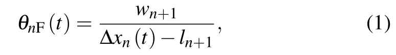
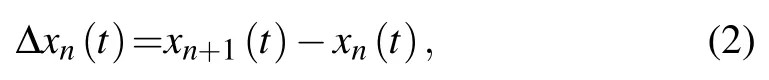
where θnF(t) means the visual angle formed by the n-th car and the car in front of it,wn+1is the width of leading vehicle and ln+1is the length of leading vehicle. Δxn(t)is the distance between n-th car and its leading car at time t. The calculation formula is as follows:

Similarly, the formula for calculating the visual angle of following vehicle(the(n−1)-th vehicle)relative to the target vehicle can be expressed as follows:

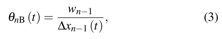
where θnB(t) means the visual angle formed by the n-th car and the car behind it and wn−1is the width of the following vehicle.

The driver optimizes the speed according to the visual angle of front and rear vehicles;therefore,the optimized velocity function can be expressed as follows:

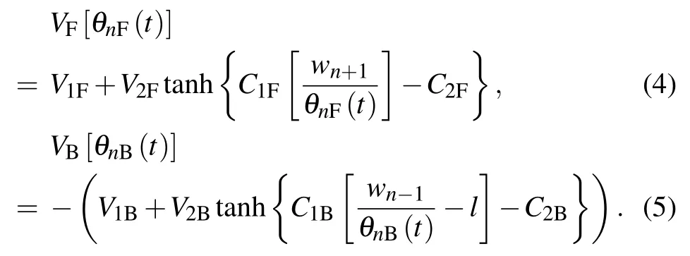
Equation (4) shows the optimal velocity function determined by the forward visual information, while equation (5)shows the optimal velocity function determined by the backward visual information. V1F, V2F, C1F, C2F, V1B, V2B, C1B,and C2Bare the parameters of optimal velocity function to be calibrated. The values are V1F=V1B=6.75 m/s,V2F=V2B=7.91 m/s,C1F=C1B=0.13 m−1,C2F=C2B=1.57.

Equations(4)and(5)show that the expressions of VBand VFare almost the same. The main difference is the difference in overall value direction because the influence of backwardlooking and forward-looking effects on car-following behavior is opposite.For example,when the front car is close to the current car,the forward visual angle increases,and the current car will respond to deceleration. When the rear car is close to the current car,the rear visual angle will also increase,but the current car will respond to acceleration.The reason why the same optimal velocity function as the function in previous work is adopted is to contrast the new model with the FVD model directly.It is perfectly acceptable to assume the optimal velocity function of other forms rather than the form of headway, but then the parameters must be recalibrated.

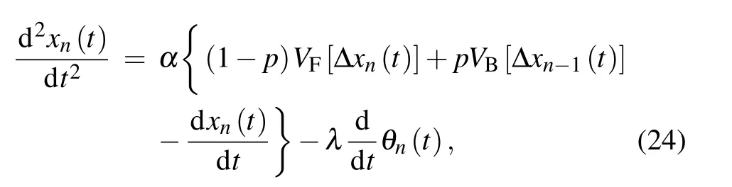
Combining the influence of optimized velocity of front and rear vehicles and the rate of change of visual angle, the car-following model under the influence of backward-looking effect can be expressed as follows:

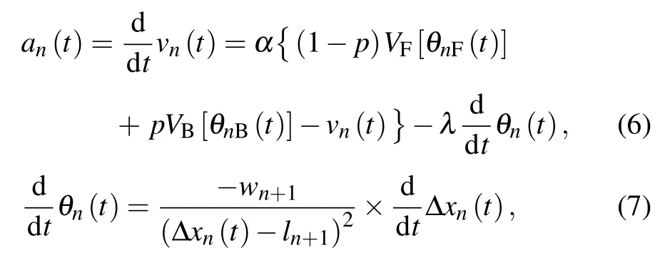
where p is the parameter of influencing factors of backwardlooking effect. When p=0, the driver is not influenced by backward-looking effect;α is the sensitivity coefficient,which is the reciprocal of reaction time τ;λ is the response intensity coefficient to the stimulation of visual angle change rate. The value of λ is larger than α, which need to be explained as follows. Firstly,the value of λ is derived according to the calibration of the actual driving data(from NGSIM)and the general range is 40-60, which is not set casually. Secondly, the value of λ is unable to decide whether the changing rate of visual angle(as shown in Eq.(7))can be neglected. Particularly,in the case of the relatively small headway, the changing rate of the forward visual angle can get large, which affected the acceleration deeply. Thirdly, the changing rate of visual angle is used as the parameter influencing acceleration and has a significant influence on the stability analysis result.

Equation(6)describes the calculation method of acceleration of target vehicle with the front and rear vehicle visual angle information as the stimulus factor. The optimized velocity in the model is obtained from the weighted average of optimized velocities decided by the forward and backward visual angles,i.e.,the driver can obtain the optimal velocity based on the forward and backward visual angle information at the same time and adjust his or her own speed. Essentially, this model indicates that the driver comprehensively considers the visual angle information of front and rear vehicles and tries to maintain the same visual angle forwards and backwards to maintain the stability of headway. When p=0, the backward-looking effect completely disappears, and the model is simplified to only consider the leading car.[28]

3. Linear stability analysis

The stability of car-following model is one of its important characteristics. The propagation law of density waves in a traffic flow can be obtained by analyzing the stability of carfollowing model, which has great significance for analyzing the formation mechanism of traffic congestion and proposing related improvement measures.

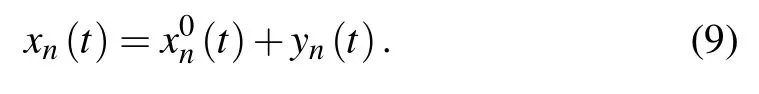
Suppose that the initial operating state of vehicle is stable,i.e., the headway is h (h=L/N, L is the total length of road and N is the total number of vehicles), and all the cars maintain the same velocity,the optimized velocity(1−p)VF(θ0F)+pVB(θ0B). Then,the initial position of each vehicle is

At this time, a small disturbance yn(t) is applied in the traffic flow so that the vehicle position changes from the steady state,written as

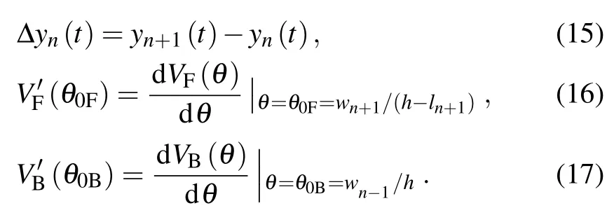
And the headway can be expressed as follows:

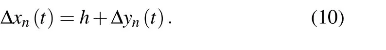
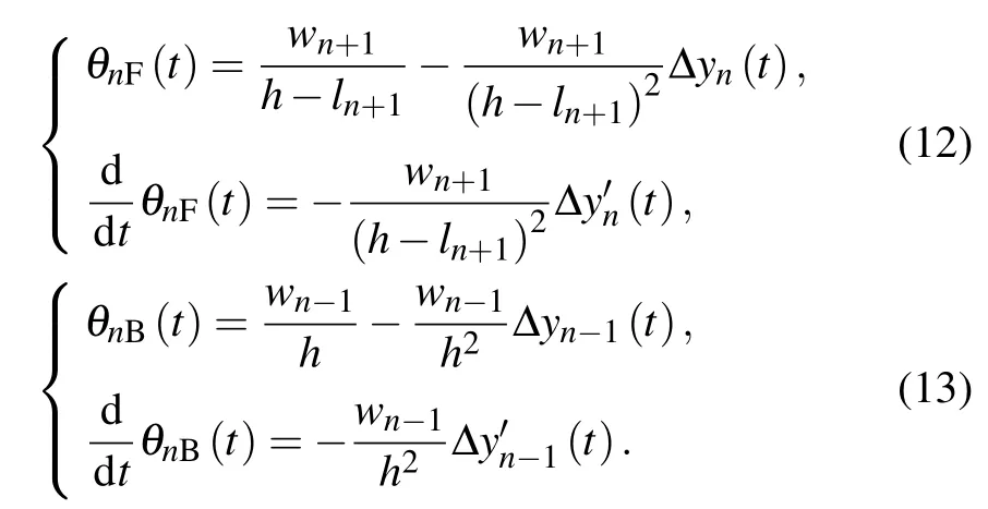
By substituting Eq. (10) into Eqs. (1) and (3), the front and rear visual angles can be calculated as follows:

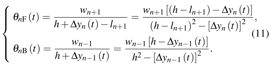
Because yn(t)is very small,its quadratic term is ignored.The rate of change of visual angle can be obtained by the derivation of θnF(t)and θnB(t):

By substituting the above two sets of expressions into Eq.(6)and linearizing the optimized velocity function by Taylor expansion

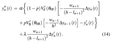
Thus,

The small disturbance yn(t) can be expressed with Fourier mode as follows:

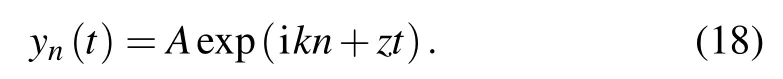
The first and second derivatives can be calculated and substituted into Eq.(14)

z can be expanded as follows:

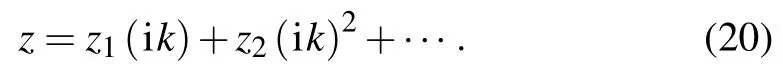
By substituting z into Eq.(19),we have

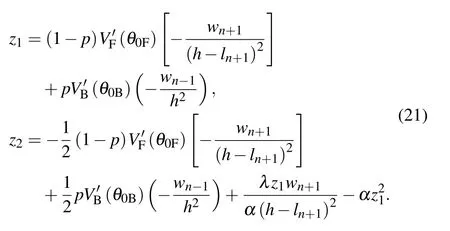
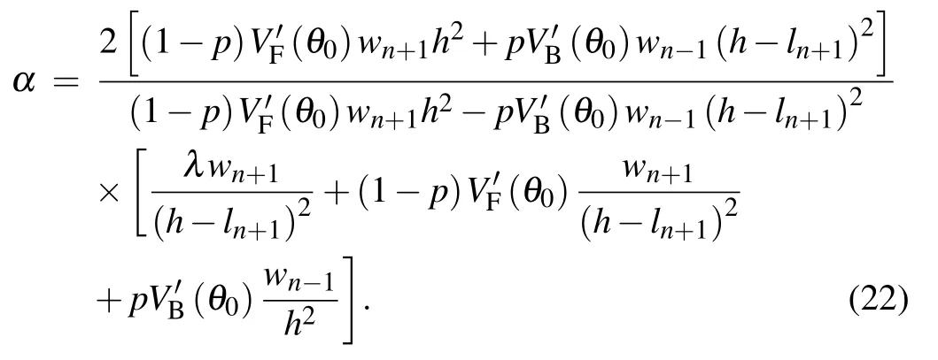
Let z2=0,and the critical condition of linear stability of the model is

When z2＞0, the traffic flow will gradually return to a stable state under the influence of small disturbance, so the condition that makes the model in a linear stable state is

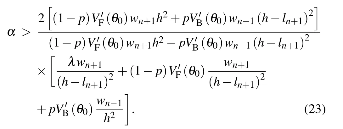
Figure 2 shows the stability critical curve of the model under different conditions, presenting the relationship between sensitivity coefficient and headway. The four solid lines in Fig.2(a)from the top to the bottom are the critical curves obtained by linear analysis with the conditions λ =20, 40, 60,80,and the values of p are all 0.2. In Fig.2(b),the four solid lines from the top to the bottom are the critical curves obtained by linear analysis with the conditions p=0.2,0.1,0.05,0,and all the λ values are 40. The whole plot is divided into upper and lower regions by the curve. The stable region is above the curve,and its characteristic is that the traffic flow can run stably without obstruction. The unstable area is under the curve,and its characteristic is that a stop-and-go phenomenon will appear in the traffic stream with the gradual expansion of small disturbance.

Each curve in Fig.2 has a vertex,which is a critical point.Multiple curves indicate that the critical point is different under different parameter conditions. For the critical sensitivity coefficient αc, when α ＞αc, i.e., the driver’s sensitivity is high,and the sensitivity coefficient is greater than the critical value. Thus, the traffic flow can be smoothly maintained regardless of the headway. If α ＜αc, the state of traffic flow mainly depends on the headway. Taking the critical headway as a reference,increase or decrease of the headway will reduce the requirement for the sensitivity coefficient, and the traffic flow will more easily enter a stable state. When the headway is near the critical value hc,the sensitivity coefficient must be increased to αcto ensure the stability of traffic flow.

Figure 2(a)shows that with the increase of λ,the movement direction of critical point is generally downward and slightly to the right, indicating that the critical headway is slightly increased,the critical sensitivity coefficient is reduced to a large extent, and the stable area in the figure becomes larger, i.e., the driver’s attention is more concentrated. When the driver is more sensitive to changes in visual angle, it becomes easier for the traffic flow to reach a stable state. As the value of p decreases in Fig.2(b),the critical point moves to the upper left, the headway decreases, and the critical sensitivity coefficient increases, indicating that the degree of consideration of rear-view effect is gradually reduced. This will make it more difficult for traffic flow to run in a stable state at a high density.

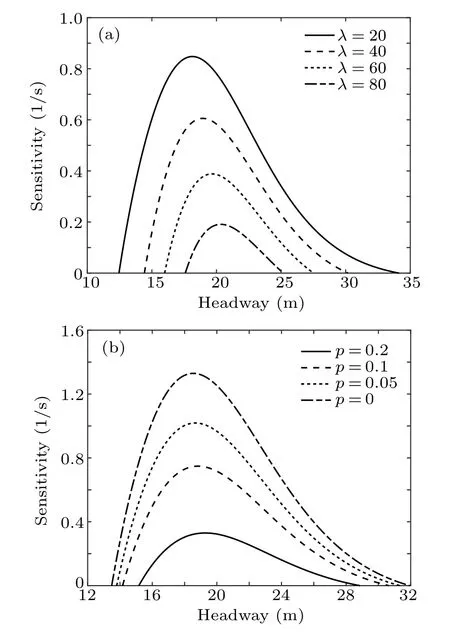
Fig.2. Linear critical curves of different parameters: different λ (a) and different p(b).

Figure 3 compares the linear stability of critical curves of different models. Except for the FVD model,[8]all other models consider the influence of backward-looking effect.The stability curves of BLVD model[21]and BL&OVC model[31]almost coincide when the critical headway is consistent, indicating that these models did not substantially improve the stability conditions. When the headway is small, the stability region formed by the stability curve of model proposed in this study is relatively large,indicating that the driver is more concerned about the behavior of rear car in a congested state and uses its behavior as a basis to adjust the speed to avoid collisions.

Fig.3. Critical curves of different models.

4. Nonlinear stability analysis

Nonlinear analysis is widely used in the field of nonlinear systems. In order to analyze the nonlinear characteristic of the new model describing the co-effect of forward and backward visual angle, we research on its gradually changing behavior for long waves of time and space variables around the critical point(αc,hc)using the mKdV equation.

To do a relatively simple calculation,we use the VF[xn(t)]and VB[xn(t)] to take the place of VF[θn(t)] and VB[θn(t)] respectively and equation(6)can be converted to the following equation:

then we can gain the expression of the(n+1)-th car further

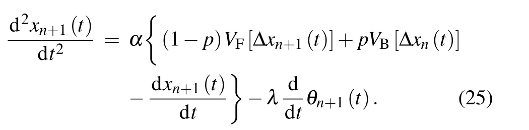
Subtract Eq.(24)from Eq.(25)and we can derive

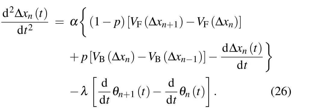
The condition α =αcis satisfied near the critical point and we define the slow variables X and T as follows using the space variable n and the time variable t in the range 0 ＜ε ≤1.

Thereinto, b is a constant coefficient undetermined and we assume that the headway between two cars is

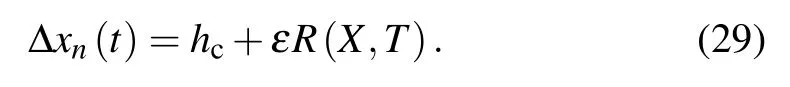
Expanding Eq. (26) in Taylor’s series and taking to the fifth term of ε,we can get the following equation:

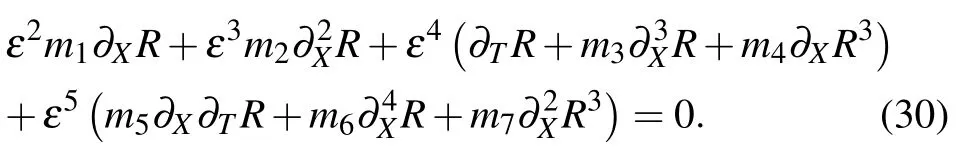
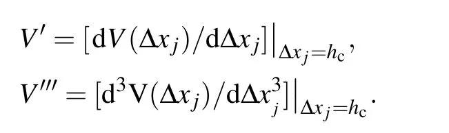
The expressions of parameters mi(i=1,2,3,4,5,6,7)are

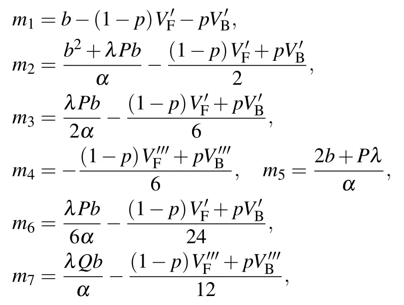
where

Here P and Q are constants which are expressed as P=−wn+1/(hc−ln+1)2and Q=−3wn+1/(hc−ln+1)4.

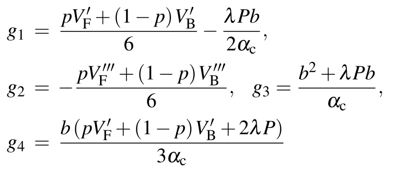
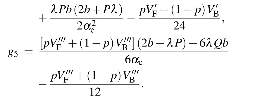
Thereinto,the expression of gi(i=1,2,3,4,5)can be written as follows by calculation:

As we can see in the following equation, the variables are supposed to be converted to another form and the purpose of the transformation is to derive the modified KdV equation which is with infinitesimal of higher orders.

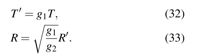
Then we deduce the following regularized equation

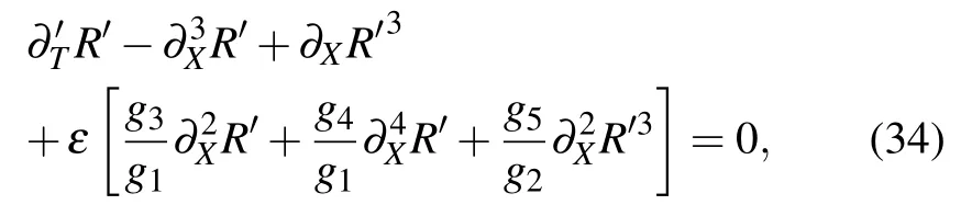
which includes the correction term O(ε). What we do next is ignoring the term O(ε)to get further the mKdV equation with the kink-antikink soliton solution

Then we assume and reconsider the O(ε)correction term. As a result, the propagation speed c can be composed of the parameters gi

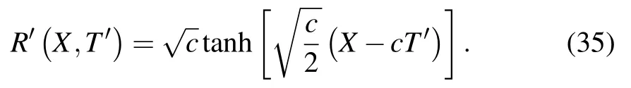
Therefore, the kink-antikink soliton solution of the headway is expressed in the following form

the amplitude of the solution is equal to

The expressions Δx=hc+A and Δx=hc−A represent the headways of two opposite phases, the low-density free flow phase and the high-density congested phase. The two mentioned phases can be combined into one coexisting phase which can be indicated by the kink-antikink soliton solution.Consequently,we achieve our goal of depicting the traffic flow state around the critical point(αc,hc)adopting the solution of the mKdV equation.

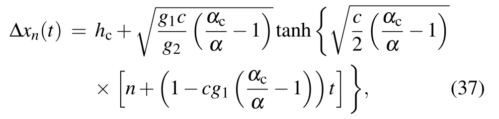
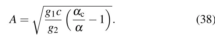
In Fig.4, the black curves are the linear stability critical curves and the red curves with the same relative line style are the nonlinear stability critical curves. Obviously,the addition of nonlinear stability critical curves under the same conditions divides the whole picture into three regions, namely, the stable region(the common region above the two curves under the same conditions), the metastable region (the region between the two curves) and the unstable region (the common region below the two curves). Since the driver’s behavior is asymmetrical in the process of acceleration and deceleration, the nonlinear stability curves show the characteristics of asymmetry which is similar to the linear stability curves.

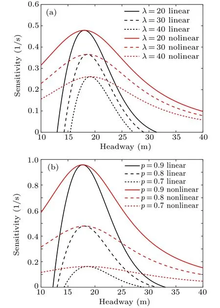
Fig.4. Linear critical curves of different parameters: different λ (a) and different p(b).

5. Numerical simulation

To further illustrate that the introduction of rear-view effect can more accurately describe the real driving behavior and its spatial and temporal evolution, the model characteristics were analyzed in depth by numerical simulation. In the simulation,all vehicles have the same size: The length is l=5 m,and the width is w=1.8 m. A periodic boundary condition is set as the length of ring road L=1500,and the total number of vehicles N =100. The initial state is stable, i.e., the vehicles are evenly distributed,and the running velocity is the same. In the initial state, the initial position of the first car is 1, indicating that a small disturbance is applied to the first car. The initial state of the vehicles can be expressed as follows:

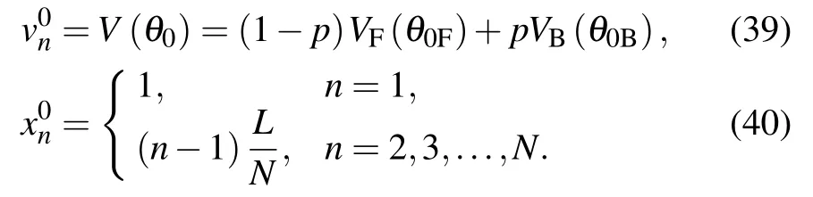
The running state parameters of the vehicles can be expressed as follows:

This section aims to verify the effect of different factors by setting different experimental conditions to prove that the proposed model can further enhance the stability of traffic flow by considering the forward and backward vision effects.

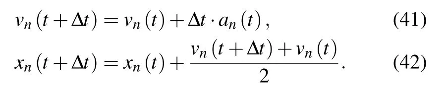
Figure 5 shows the position distribution of each car under different values of p for a period after the disturbance is applied. The period is selected as t=2000 s-2200 s; p is 0,0.1,0.2, and 0.3; λ is 5, and other parameters remain the same.The aim is to directly analyze the influence of rate of change of visual angle in the model. In the three pictures shown in Figs. 5(a)-5(c), the uneven distribution of vehicles can be clearly observed,showing that the vehicles on the ring road are sparsely or densely distributed on different road sections,i.e.,the stop-and-go phenomena. Beyond that, with the increase of p,the driver’s visual perception of rear car becomes strong,and the degree of sparse or dense lines of the vehicle gradually slows down. The width and number of stripes that can describe the traffic congestion decrease,i.e.,the region of congestion becomes smaller,and the stop-and-go phenomenon is alleviated. When p=0.3, i.e., the stability condition is satisfied, the disturbance of traffic flow disappears after 2000 s,the headway between vehicles remains equal and unchanged,and the traffic flow enters a stable state. This shows that it can effectively enhance the stability of traffic flow for the driver to adjust the observation ratio of forward and backward information to a certain extent.

Because the model proposed in this study can describe the effect of different car sizes on the driver’s rear-view effect, it was considered to add large cars and set different proportions in the simulation process. The size of a large car was set to 5-m long and 2.5-m wide. In the simulation,the proportion of large vehicles was set to 0.2, 0.1, 0.05, and 0.02; λ is 10; p is 0.2; other parameters were kept the same. Figure 6 shows the change trend of vehicle headway under different proportions of large vehicles after a disturbance is applied. The time points of the two figures are t=300 s and t=2000 s. Figure 6 shows that with the increase in the proportion of large vehicles, the amplitude of up and down fluctuations of headway decreases, and the stop-and-go phenomenon gradually slows down. This indicates that the stability of traffic flow can be improved if there is a certain proportion of large vehicles on the road, whether the large vehicle is observed as the leading car or the rear car because large cars can increase the driver’s attention and sensitivity to changes in their behavior.

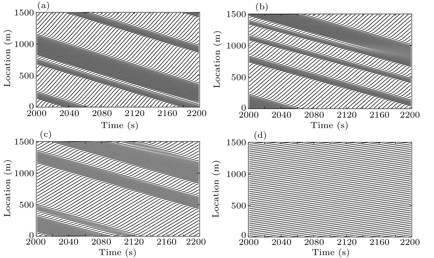
Fig.5. Spatiotemporal vehicle trajectory diagrams for different values of p: (a) p=0,(b) p=0.1,(c) p=0.2,and(d) p=0.3.

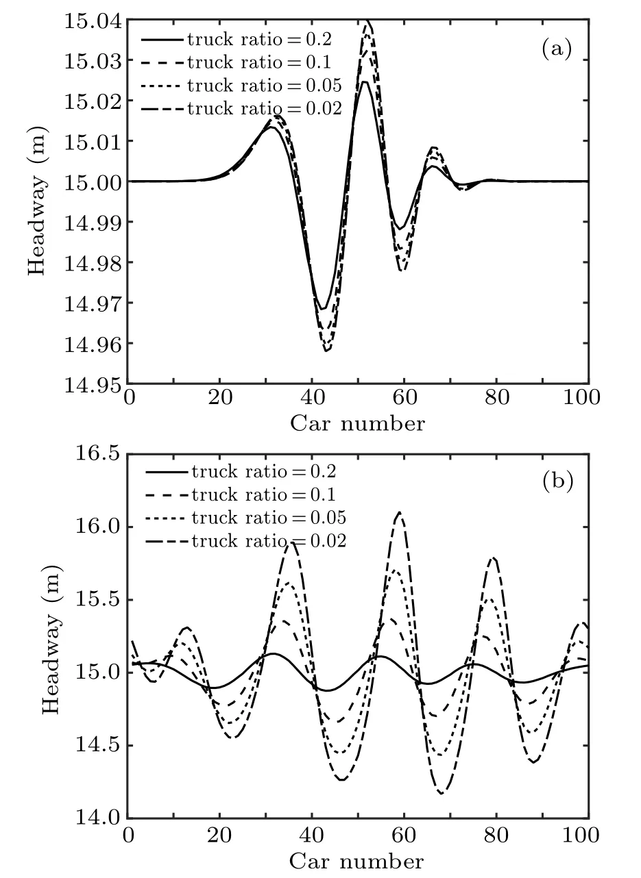
Fig.6. Stop-and-go waves of different truck ratios: (a) t = 300 s, (b)t=2000 s.

Because there are certain differences in the driving habits of drivers,there will be different decisions on whether to consider the backward-looking effect. Figure 7 shows the spatial and temporal evolution of a headway within a period after the disturbance is applied under different vehicle proportions considering the backward-looking effect. In the simulation, the proportion of vehicles considering the backward-looking effect was set to 0, 0.5, 0.8, and 0.95; the p value is 0.25; the λ value is 5; other parameters were also consistent. All the curves in the three graphs of Figs.7(a)-7(c)fluctuate significantly,indicating that the traffic flow is unstable. In Fig.7(a),all vehicles are only influenced by the front visual angle. The headway greatly fluctuates in the traffic flow. The vehicle is in a stop-and-go state, and the traffic flow is congested. In Fig.7(b),the number of vehicles that only considers the front visual angle and the number of the vehicles that considers both the front and rear visual information make up half of the total number of vehicles. There is still a large fluctuation in the headway. The distribution of headway is discontinuous and varies between two sets of similar data.Such a ratio makes the situation of traffic flow more complex.In Fig.7(c),the ratio of vehicles considering front and rear visual information simultaneously is 80%. The distance between the heads still fluctuates,but the amplitude is significantly reduced compared to the previous two cases. An uneven distribution phenomenon still exists, but it is obviously alleviated. The traffic flow tends to be more stable. In Fig.7(d),95%of the vehicles consider both the front and rear visual information. The head-to-head distance remains unchanged. The small fluctuations are caused by a small number of vehicles that only observe the vehicle in front. The traffic flow is basically stable. Based on the above analysis, the influence of driver’s perception of the rear-view effect on car-following behavior can promote the stability of the traffic flow.This also provides a basis for building an intelligent vehicle control model with the traffic flow stabilization.

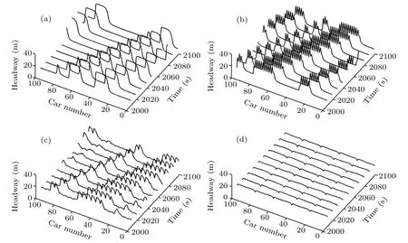
Fig.7. Spatiotemporal evolution of distance headway considering different proportions of visual information forward and backward: (a)rate=0,(b)rate=0.5,(c)rate=0.8,(d)rate=0.95.

6. Conclusion

This study fully considers the characteristics of driver’s corresponding car-following behavior by visually acquiring the front and rear vehicle information during driving, introduces a concept of visual angle to describe the visual stimuli of front and rear vehicles,and proposes a car-following model under the influence of rear-view.Through linear stability analysis, a critical stability condition of the model was obtained.The stable area of traffic flow can be expanded by increasing the driver’s sensitivity to the rate of change of visual angle and increasing the ratio of considering the backward-looking effect. The result of nonlinear stability analysis is consistent with that of linear stability analysis. Using numerical simulation to further analyze the characteristics of the model, the results show that different parameter settings, different sizes of large vehicles,and the proportion of backward-looking effects have a significant effect on the spatiotemporal evolution of traffic flow. Therefore, consideration of the visual characteristics of human driver in the model can be closer to the real situation. The driver observes the traffic conditions forwards and backwards with a reasonable allocation ratio and then makes driving decisions,conducive to the stability of traffic flow. This study also provides a basis for studying vehicle control rules in an intelligent networked environment.