Multiagent Reinforcement Learning:Rollout and Policy Iteration

Dimitri Bertsekas

Abstract—We discuss the solution of complex multistage decision problems using methods that are based on the idea of policy iteration (PI), i.e., start from some base policy and generate an improved policy. Rollout is the simplest method of this type,where just one improved policy is generated. We can view PI as repeated application of rollout, where the rollout policy at each iteration serves as the base policy for the next iteration.In contrast with PI, rollout has a robustness property: it can be applied on-line and is suitable for on-line replanning. Moreover,rollout can use as base policy one of the policies produced by PI, thereby improving on that policy. This is the type of scheme underlying the prominently successful AlphaZero chess program.

I. INTRODUCTION

IN this paper we discuss the solution of large and challenging multistage decision and control problems, which involve controls with multiple components,each associated with a different decision maker or agent.We focus on problems that can be solved in principle by dynamic programming (DP),but are addressed in practice using methods of reinforcement learning (RL), also referred to by names such as approximate dynamic programming and neuro-dynamic programming. We will discuss methods that involve various forms of the classical method of policy iteration(PI),which starts from some policy and generates one or more improved policies.

If just one improved policy is generated, this is called rollout, with the initial policy called base policy and the improved policy called rollout policy. Based on broad and consistent computational experience, rollout appears to be one of the simplest and most reliable of all RL methods(we refer to the author’s textbooks [1]−[3] for an extensive list of research contributions and case studies on the use of rollout). Rollout is also well-suited for on-line model-free implementation and on-line replanning.

Approximate PI is one of the most prominent types of RL methods. It can be viewed as repeated application of rollout, and can provide (off-line) the base policy for use in a rollout scheme. It can be implemented using data generated by the system itself, and value and policy approximations.Approximate forms of PI, which are based on the use of approximation architectures, such as value and policy neural networks, have most prominently been used in the spectacularly successful AlphaZero chess program; see Silver et al. [4]. In particular, in the AlphaZero architecture a policy is constructed via an approximate PI scheme that is based on the use of deep neural networks. This policy is used as a base policy to generate chess moves on-line through an approximate multistep lookahead scheme that applies Monte Carlo tree search with an approximate evaluation of the base policy used as a terminal cost function approximation.Detailed descriptions of approximate PI schemes can be found in most of the RL textbooks, including the author’s[2], [3], which share the notation and point of view of the present paper.

1) Our Multiagent Structure

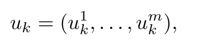
The purpose of this paper is to survey variants of rollout and PI for DP problems involving a control u at each stage that consists of multiple components u1,...,um, i.e.,

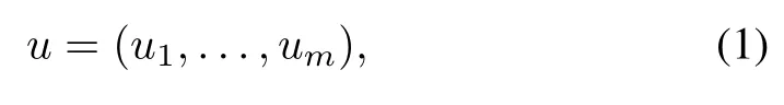
where the components uℓare selected independently from within corresponding constraint sets Uℓ, ℓ = 1,...,m. Thus the overall constraint set is u ∈U, where U is the Cartesian product1We will also allow later dependence of the sets Uℓ on a system state.More complex constraint coupling of the control components can be allowed at the expense of additional algorithmic complications; see [3], [5], [6].

We associate each control component uℓwith the ℓth of m agents.

The term “multiagent” is used widely in the literature,with several different meanings. Here, we use this term as a conceptual metaphor in the context of problems with the multi-component structure(1);it is often insightful to associate control components with agent actions. A common example of a multiagent problem is multi-robot (or multi-person)service systems, often involving a network, such as delivery,maintenance and repair,search and rescue,firefighting,taxicab or utility vehicle assignment, and other related contexts. Here the decisions are implemented collectively by the robots (or persons, respectively), with the aid of information exchange or collection from sensors or from a computational “cloud.”The information may or may not be common to all the robots or persons involved. Another example involves a network of facilities, where service is offered to clients that move within the network. Here the agents may correspond to the service facilities or to the clients or to both, with information sharing that may involve errors and/or delays.

Note, however, that the methodology of this paper applies generally to any problem where the control u consists of m components, u = (u1,...,um) [cf. Eq.(1)], independently of the details of the associated practical context. In particular,the practical situation addressed may not involve recognizable“agents” in the common sense of the word, such as multiple robots, automobiles, service facilities,or clients. For example,it may simply involve control with several components, such as a single robot with multiple moving arms, a chemical plant with multiple interacting but independently controlled processes,or a power system with multiple production centers.

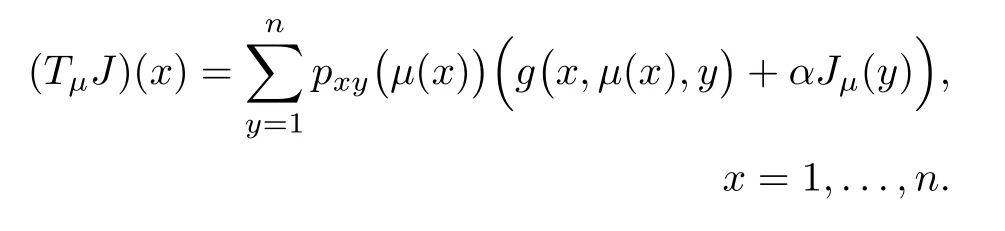
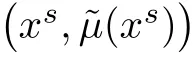
As is generally true in DP problems, in addition to control,there is an underlying state, denoted by x, which summarizes all the information that is useful at a given time for the purposes of future optimization. It is assumed that x is perfectly known by all the agents at each stage.2Partial observation Markov decision problems(POMDP)can be converted to problems involving perfect state information by using a belief state;see e.g.,the textbook [1]. Our assumption then amounts to perfect knowledge of the belief state by all agents. For example, we may think of a central processing computational “cloud” that collects and processes state information, and broadcasts a belief state to all agents at each stage.In a PI infinite horizon context,given the current policyµ[a function that maps the current state x to an m-component controlµ(x) =(µ1(x),...,µm(x)), also referred to as the base policy], the policy improvement operation portion of a PI involves at each state x, a one-step lookahead minimization of the general form

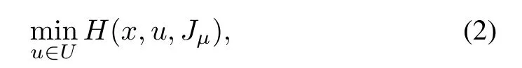
where Jµis the cost function of policy µ (a function of x), and H is a problem-dependent Bellman operator. This minimization may be done off-line(before control has started)or on-line (after control has started), and defines a new policy ˜µ (also referred to as the rollout policy), whereby the control ˜µ(x) to be applied at x is the one attaining the minimum above. The key property for the success of the rollout and PI algorithms is the policy improvement property

i.e., the rollout policy yields reduced cost compared with the base policy, for all states x. Assuming that each set Uℓis finite (as we do in this paper), there are two difficulties with the lookahead minimization (2), which manifest themselves both in off-line and in on-line settings:

(a) The cardinality of the Cartesian product U grows exponentially with the number m of agents, thus resulting in excessive computational overhead in the minimization over u ∈U when m is large.

(b) To implement the minimization (2), the agents need to coordinate their choices of controls, thus precluding their parallel computation.

In this paper, we develop rollout and PI algorithms, which,as a first objective, aim to alleviate the preceding two difficulties. A key idea is to introduce a form of sequential agent-by-agent one-step lookahead minimization, which we call multiagent rollout. It mitigates dramatically the computational bottleneck due to (a) above. In particular, the amount of computation required at each stage grows linearly with the number of agents m, rather than exponentially. Despite the dramatic reduction in required computation, we show that our multiagent rollout algorithm has the fundamental cost improvement property (3): it guarantees an improved performance of the rollout policy relative to the base policy.

Multiagent rollout in the form just described involves coordination of the control selections of the different agents.In particular, it requires that the agents select their controls sequentially in a prespecified order,with each agent communicating its control selection to the other agents.To allow parallel control selection by the agents [cf. (b) above], we suggest to implement multiagent rollout with the use of a precomputed signaling policy that embodies agent coordination. One possibility is to approximately compute off-line the multiagent rollout policy through approximation in policy space,i.e.,training an approximation architecture such as a neural network to learn the rollout policy. This scheme, called autonomous multiagent rollout, allows the use of autonomous, and faster distributed and asynchronous on-line control selection by the agents, with a potential sacrifice of performance, which depends on the quality of the policy space approximation.Note that autonomous multiagent rollout makes sense only in the context of distributed computation. If all computations are performed serially on a single processor, there is no reason to resort to signaling policies and autonomous rollout schemes.

Let us also mention that distributed DP algorithms have been considered in a number of contexts that involve partitioning of the state space into subsets, with a DP algorithm executed in parallel within each subset. For example distributed value iteration has been investigated in the author’s papers [7], [8], and the book [9]. Also asynchronous PI algorithms have been discussed in a series of papers of the author and Yu[10]−[12],as well as the books[3],[13],[14].Moreover,distributed DP based on partitioning in conjunction with neural network training on each subset of the partition has been considered in the context of a challenging partial state information problem by Bhattacharya et al. [15]. The algorithmic ideas of these works do not directly apply to the multiagent context of this paper. Still one may envision applications where parallelization with state space partitioning is combined with the multiagent parallelization ideas of the present paper.In particular,one may consider PI schemes that involve multiple agents/processors, each using a state space partitioning scheme with a cost function and an agent policy defined over each subset of the partition.The agents may then communicate asynchronously their policies and cost functions to other agents, as described in the paper [10] and book[3] (Section 5.6), and iterate according to the agent-by-agent policy evaluation and policy improvement schemes discussed in this paper. This, however, is beyond our scope and is left as an interesting subject for further research.

2) Classical and Nonclassical Information Patterns

It is worth emphasizing that our multiagent problem formulation requires that all the agents fully share information,including the values of the controls that they have applied in the past, and have perfect memory of all past information.This gives rise to a problem with a so called “classical information pattern,”a terminology introduced in the papers by Witsenhausen [16], [17]. A fact of fundamental importance is that problems possessing this structure can be addressed with the DP formalism and approximation in value space methods of RL. Problems where this structure is absent, referred to as problems with “nonclassical information pattern,” cannot be addressed formally by DP (except through impractical reformulations), and are generally far more complicated, as illustrated for linear systems and quadratic cost by the famous counterexample of [16].

Once a classical information pattern is adopted, we may assume that all agents have access to a system state3The system state at a given time is either the common information of all the agents, or a sufficient statistic/summary of this information, which is enough for the computation of a policy that performs arbitrarily close to optimal. For example in the case of a system with partial state observations,we could use as system state a belief state; see e.g., [1].and make use of a simple conceptual model: there is a computational“cloud” that collects information from the agents on-line,computes the system state, and passes it on to the agents,who then perform local computations to apply their controls as functions of the system state; see Fig.1. Alternatively,the agent computations can be done at the cloud, and the results may be passed on to the agents in place of the exact state. This scheme is also well suited as a starting point for approximations where the state information made available to the agents is replaced by precomputed“signaling”policies that guess/estimate missing information. The estimates are then treated by the agents as if they were exact. Of course such an approach is not universally effective, but may work well for favorable problem structures.4For example consider a problem where the agent locations within some two-dimensional space become available to the other agents with some delay.It may then make sense for the agents to apply some algorithm to estimate the location of the other agents based on the available information, and use the estimates in a multiagent rollout scheme as if they were exact.Its analysis is beyond the scope of the present paper, and is left as a subject for further research.

Fig.1. Illustration of a conceptual structure for our multiagent system. The“cloud” collects information from the environment and from the agents online, and broadcasts the state (and possibly other information) to the agents at each stage, who then perform local computations to apply their controls as functions of the state information obtained from the cloud. Of course some of these local computations may be done at the cloud, and the results may be passed on to the agents in place of the exact state.In the case of a problem with partial state observation, the cloud computes the current belief state (rather than the state).

We note that our multiagent rollout schemes relate to a well-developed body of research with a long history: the theory of teams and decentralized control, and the notion of person-by-person optimality; see Marschak [18], Radner[19], Witsenhausen [17], [20], Marschak and Radner [21],Sandell et al. [22], Yoshikawa [23], Ho [24]. For more recent works,see Bauso and Pesenti[25],[26],Nayyar,Mahajan,and Teneketzis [27], Nayyar and Teneketzis [28], Li et al. [29],Qu and Li [30], Gupta [31], the books by Bullo, Cortes, and Martinez [32], Mesbahi and Egerstedt [33], Mahmoud [34],and Zoppoli, Sanguineti, Gnecco, and Parisini [35], and the references quoted there.

The connection of our work with team theory manifests itself in our infinite horizon DP methodology, which includes value iteration and PI methods that converge to a person-byperson optimal policy. Note that in contrast with the present paper, a large portion of the work on team theory and decentralized control allows a nonclassical information pattern,whereby the agents do not share the same state information and/or forget information previously received, although they do share the same cost function. In the case of a multiagent system with partially observed state, this type of model is also known as a decentralized POMDP (or Dec-POMDP), a subject that has attracted a lot of attention in the last 20 years;see e.g., the monograph by Oliehoek and Amato [36], and the references quoted there. We may also note the extensive literature on game-theoretic types of problems,including Nash games,where the agents have different cost functions;see e.g.,the surveys by Hernandez-Leal et al. [37], and Zhang, Yang,and Basar [38]. Such problems are completely outside our scope and require a substantial departure from the methods of this paper.Zero-sum sequential games may be more amenable to treatment with the methodology of this paper, because they can be addressed within a DP framework (see e.g., Shapley[39], Littman [40]), but this remains a subject for further research.

In addition to the aforementioned works on team theory and decentralized control,there has been considerable related work on multiagent sequential decision making from a machine learning perspective, often with the use of variants of policy gradient, Q-learning, and random search methods. Works of this type also have a long history,and they have been surveyed over time by Sycara [41], Stone and Veloso [42], Panait and Luke [43], Busoniu, Babuska, and De Schutter [44],[45], Matignon, Laurent, and Le Fort-Piat [46], Hernandez-Leal, Kartal, and Taylor [47], OroojlooyJadid and Hajinezhad[48], Zhang, Yang, and Basar [38], and Nguyen, Nguyen,and Nahavandi [49], who list many other references. For some representative recent research papers, see Tesauro [50],Oliehoek, Kooij, and Vlassis [51], Pennesi and Paschalidis[52], Paschalidis and Lin [53], Kar, Moura, and Poor [54],Foerster et al. [55], Omidshafiei et al. [56], Gupta, Egorov,and Kochenderfer [57], Lowe et al. [58], Zhou et al. [59],Zhang et al. [60], Zhang and Zavlanos [61], and de Witt et al. [62].

These works collectively describe several formidable difficulties in the implementation of reliable multiagent versions of policy gradient and Q-learning methods,although they have not emphasized the critical distinction between classical and nonclassical information patterns. It is also worth noting that policy gradient methods, Q-learning, and random search are primarily off-line algorithms, as they are typically too slow and noise-afflicted to be applied with on-line data collection.As a result, they produce policies that are tied to the model used for their training. Thus, contrary to rollout, they are not robust with respect to changes in the problem data, and they are not well suited for on-line replanning. On the other hand,it is possible to train a policy with a policy gradient or random search method by using a nominal model, and use it as a base policy for on-line rollout in a scheme that employs on-line replanning.

3) Related Works

The multiagent systems field has a long history, and the range of related works noted above is very broad. However,while the bottleneck due to exponential growth of computation with the number of agents has been recognized [47], [48], it has not been effectively addressed. It appears that the central idea of the present paper, agent-by-agent sequential optimization while maintaining the cost improvement property, has been considered only recently. In particular, the approach to maintaining cost improvement through agent-by-agent rollout was first introduced in the author’s papers [5], [6], [63], and research monograph [3].

A major computational study where several of the algorithmic ideas of this paper have been tested and validated is the paper by Bhattacharya et al. [64]. This paper considers a large-scale multi-robot routing and repair problem, involving partial state information, and explores some of the attendant implementation issues, including autonomous multiagent rollout, through the use of policy neural networks and other precomputed signaling policies.

The author’s paper [6] and monograph [3] discuss constrained forms of rollout for deterministic problems,including multiagent forms, and an extensive range of applications in discrete/combinatorial optimization and model predictive control. The character of this deterministic constrained rollout methodology differs markedly from the one of the methods of this paper. Still the rollout ideas of the paper [6] are supplementary to the ones of the present paper, and point the way to potential extensions of constrained rollout to stochastic problems. We note also that the monograph [3] describes multiagent rollout methods for minimax/robust control, and other problems with an abstract DP structure.

4) Organization of the Paper

The present paper is organized as follows.We first introduce finite horizon stochastic optimal control problems in Section II, we explain the main idea behind the multiagent rollout algorithm, and we show the cost improvement property. We also discuss variants of the algorithm that are aimed at improving its computational efficiency. In Section III, we consider the implementation of autonomous multiagent rollout,including schemes that allow the distributed and asynchronous computation of the agents’ control components.

We then turn to infinite horizon discounted problems. In particular, in Section IV, we extend the multiagent rollout algorithm, we discuss the cost improvement property, and we provide error bounds for versions of the algorithm involving rollout truncation and simulation. We also discuss two types of multiagent PI algorithms, in Sections IV-A and IV-E,respectively. The first of these, in its exact form, converges to an agent-by-agent optimal policy, thus establishing a connection with the theory of teams. The second PI algorithm,in its exact form, converges to an optimal policy, but must be executed over a more complex state space. Approximate forms of these algorithms, as well as forms of Q-learning,are also discussed, based on the use of policy and value neural networks.These algorithms,in both their exact and their approximate form are strictly off-line methods,but they can be used to provide a base policy for use in an on-line multiagent rollout scheme. Finally, in Section V we discuss autonomous multiagent rollout schemes for infinite horizon discountedproblems, which allow for distributed on-line implementation.

II. MULTIAGENT PROBLEM FORMULATION-FINITE HORIZON PROBLEMS

We consider a standard form of an N-stage DP problem(see[1], [2]), which involves the discrete-time dynamic system

where xkis an element of some(possibly infinite)state space,the control ukis an element of some finite control space, and wkis a random disturbance,with given probability distribution Pk(· | xk,uk) that may depend explicitly on xkand uk, but not on values of prior disturbances wk−1,...,w0.The control ukis constrained to take values in a given subset Uk(xk),which depends on the current state xk. The cost of the kth stage is denoted by gk(xk,uk,wk); see Fig.2.

We consider policies of the form

π ={µ0,...,µN−1},

where µkmaps states xkinto controls uk=µk(xk), and satisfies a control constraint of the formµk(xk)∈Uk(xk)for all xk.Given an initial state x0and a policy π ={µ0,...,µN−1},the expected cost of π starting from x0is

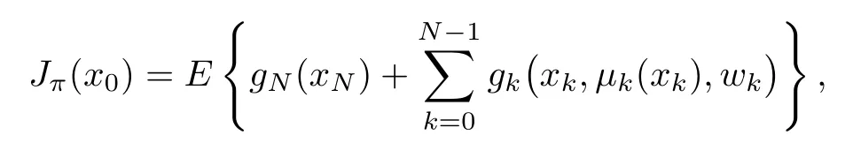
where the expected value operation E{·} is with respect to the joint distribution of all the random variables wkand xk.The optimal cost starting from x0, is defined by

where Π is the set of all policies.An optimal policy π∗is one that attains the minimal cost for every x0; i.e.,

Since the optimal cost function J∗and optimal policy π∗are typically hard to obtain by exact DP,we consider approximate DP/RL algorithms for suboptimal solution, and focus on rollout, which we describe next.

A. The Standard Rollout Algorithm and Policy Improvement

In the standard form of rollout, given a policy π ={µ0,...,µN−1},called base policy,with cost-to-go from state xkat stage k denoted by Jk,π(xk),k =0,...,N,we obtain an improved policy,i.e.,one that achieves cost that is less or equal to Jk,π(xk)starting from each xk.The base policy is arbitrary.It may be a simple heuristic policy or a sophisticated policy obtained by off-line training through the use of an approximate PI method that uses a neural network for policy evaluation or a policy gradient method of the actor/critic type (see e.g., the reinforcement learning book [2]).

The standard rollout algorithm has a long history (see the textbooks[1]−[3],[65],which collectively list a large number of research contributions). The name “rollout” was coined by Tesauro, who among others, has used a “truncated” version of the rollout algorithm for a highly successful application in computer backgammon [66]. The algorithm is widely viewed among the simplest and most reliable RL methods.It provides on-line control of the system as follows:

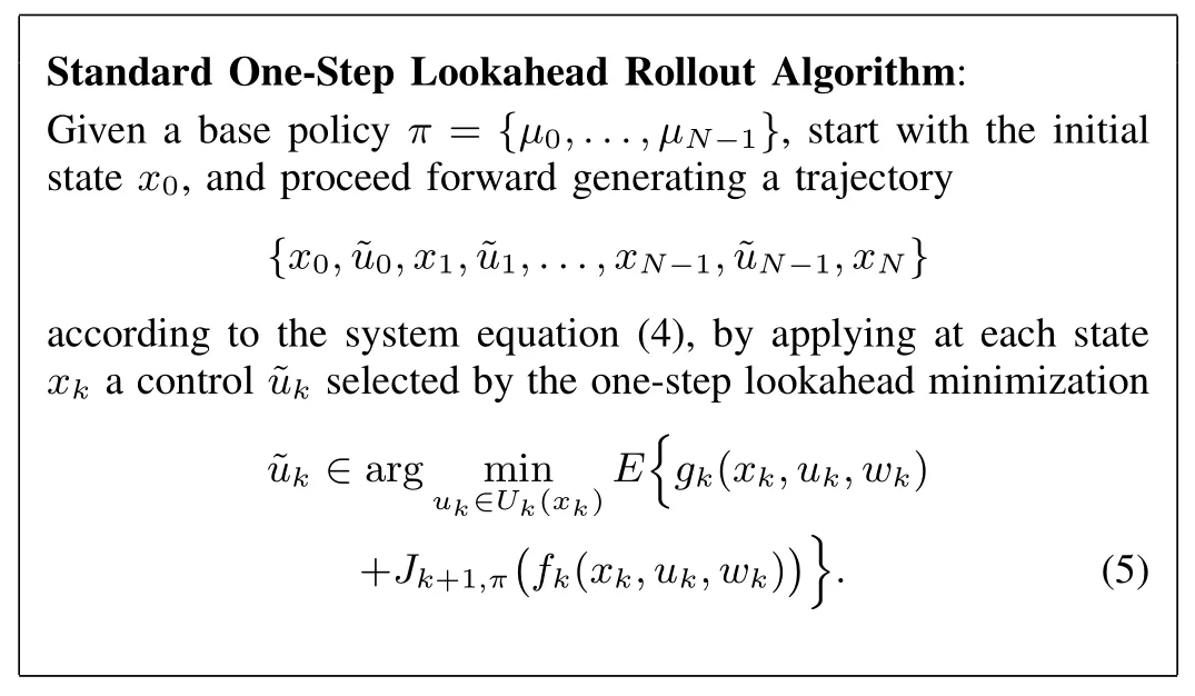
In addition to the cost improvement property, the rollout algorithm(5)has a second nice property:it is an on-line algorithm, and hence inherently possesses a robustness property:it can adapt to variations of the problem data through on-line replanning.Thus if there are changes in the problem data(such as for example the probability distribution of wk, or the stage cost function gk), the performance of the base policy can be seriously affected, but the performance of the rollout policy is much less affected because the computation in Eq.(5) will take into account the changed problem data.

Despite the advantageous properties just noted, the rollout algorithm suffers from a serious disadvantage when the constraint set Uk(xk)has a large number of elements,namely that the minimization in Eq.(5)involves a large number of alternatives.In particular,let us consider the expected value in Eq.(5),which is the Q-factor of the pair(xk,uk)corresponding to the base policy:

In the “standard” implementation of rollout, at each encountered state xk,the Q-factor Qk,π(xk,uk)is computed by some algorithm separately for each control uk∈Uk(xk) (often by Monte Carlo simulation). Despite the inherent parallelization possibility of this computation, in the multiagent context to be discussed shortly, the number of controls in Uk(xk), and the attendant computation and comparison of Q-factors, grow rapidly with the number of agents, and can become very large. We next introduce a modified rollout algorithm for the multiagent case,which requires much less on-line computation but still maintains the cost improvement property (6).

B. The Multiagent Case

We propose an alternative rollout algorithm that achieves the cost improvement property (6) at much smaller computational cost, namely of order O(qm) per stage. A key idea is that the computational requirements of the rollout one-step minimization (5) are proportional to the number of controls in the set Uk(xk) and are independent of the size of the state space. This motivates a problem reformulation, first proposed in the neuro-dynamic programming book [65], Section 6.1.4,whereby control space complexity is traded off with state space complexity by “unfolding” the control ukinto its m components,which are applied one-agent-at-a-time rather than all-agents-at-once. We will next apply this idea within our multiagent rollout context.We note,however,that the idea can be useful in other multiagent algorithmic contexts, including approximate PI, as we will discuss in Section IV-E.

C. Trading off Control Space Complexity with State Space Complexity

In Sections III and V, we will aim to relax Assumptions(b)and(c),through the use of autonomous multiagent rollout.Assumption (a) is satisfied if there is a central computation center (a “cloud”) that collects all the information available from the agents and from other sources, obtains the state (or a belief state in the case of partial state information problem),and broadcasts it to the agents as needed; cf. Fig.1. To relax this assumption, one may assume that the agents use an estimate of the state in place of the unavailable true state in all computations. However, this possibility has not been investigated and is beyond our scope.

Note that the rollout policy (8), obtained from the reformulated problem is different from the rollout policy obtained from the original problem [cf. Eq.(5)]. Generally, it is unclear how the two rollout policies perform relative to each other in terms of attained cost.On the other hand,both rollout policies perform no worse than the base policy, since the performance of the base policy is identical for both the reformulated problem and for the original problem. This is shown formally in the following proposition.

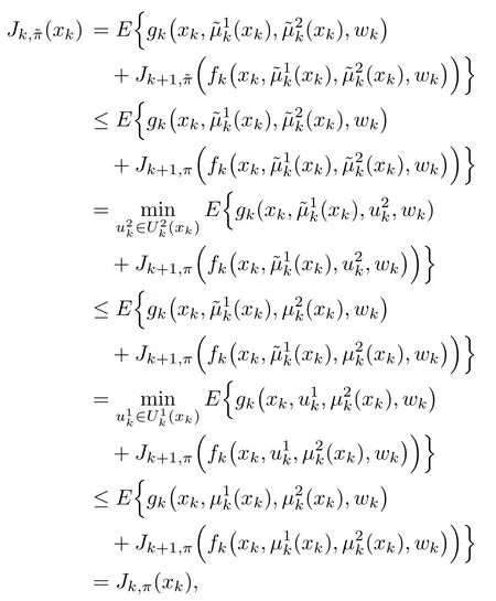
where in the preceding relation:

(b) The first inequality holds by the induction hypothesis.

(c) The second equality holds by the definition of the multiagent rollout algorithm as it pertains to agent 2.

(d) The third equality holds by the definition of the multiagent rollout algorithm as it pertains to agent 1.

(e) The last equality is the DP/Bellman equation for the base policy π.

The induction proof of the cost improvement property(9)is thus complete for the case m=2. The proof for an arbitrary number of agents m is entirely similar.■

Note that there are cases where the all-agents-at-once standard rollout algorithm can improve strictly the base policy but the one-agent-at-a-time algorithm will not.This possibility arises when the base policy is “agent-by-agent-optimal,” i.e.,each agent’s control component is optimal, assuming that the control components of all other agents are kept fixed at some known values.6This is a concept that has received much attention in the theory of team optimization, where it is known as person-by-person optimality. It has been studied in the context of somewhat different problems, which involve imperfect state information that may not be shared by all the agents; see the references on team theory cited in Section I.Such a policy may not be optimal, except under special conditions (we give an example in the next section). Thus if the base policy is agent-by-agent-optimal,multiagent rollout will be unable to improve strictly the cost function, even if this base policy is strictly suboptimal.However, we speculate that a situation where a base policy is agent-by-agent-optimal is unlikely to occur in rollout practice,since ordinarily a base policy must be reasonably simple,readily available, and easily simulated.

Let us provide an example that illustrates how the size of the control space may become intractable for even moderate values of the number of agents m.

Example 1 (Spiders and Fly)

Here there are m spiders and one fly moving on a 2-dimensional grid. During each time period the fly moves to some other position according to a given state-dependent probability distribution. The spiders, working as a team, aim to catch the fly at minimum cost (thus the one-stage cost is equal to 1, until reaching the state where the fly is caught,at which time the one-stage cost becomes 0). Each spider learns the current state (the vector of spiders and fly locations)at the beginning of each time period, and either moves to a neighboring location or stays where it is. Thus each spider ℓhas as many as five choices at each time period (with each move possibly incurring a different location-dependent cost).The control vector is u=(u1,...,um),where uℓis the choice of the ℓth spider, so there are about 5mpossible values of u.However, if we view this as a multiagent problem, as per the reformulation of Fig.4, the size of the control space is reduced to ≤5 moves per spider.

To apply multiagent rollout, we need a base policy. A simple possibility is to use the policy that directs each spider to move on the path of minimum distance to the current fly position. According to the multiagent rollout formalism, the spiders choose their moves in a given order,taking into account the current state,and assuming that future moves will be chosen ≤Jk+1,π,we have for all xk,according to the base policy. This is a tractable computation,particularly if the rollout with the base policy is truncated after some stage,and the cost of the remaining stages is approximated using a certainty equivalence approximation in order to reduce the cost of the Monte Carlo simulation.

Sample computations with this example indicate that the multiagent rollout algorithm of this section performs about as well as the standard rollout algorithm.Both algorithms perform much better than the base policy, and exhibit some “intelligence” that the base policy does not possess. In particular, in the rollout algorithms the spiders attempt to “encircle” the fly for faster capture, rather that moving straight towards the fly along a shortest path.

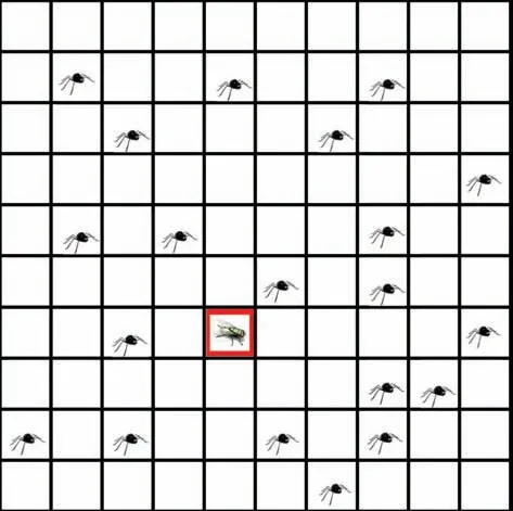
Fig.4. Illustration of the 2-dimensional spiders-and-fly problem. The state is the set of locations of the spiders and the fly. At each time period, each spider moves to a neighboring location or stays where it is. The spiders make moves with perfect knowledge of the locations of each other and of the fly.The fly moves randomly, regardless of the position of the spiders.

The following example is similar to the preceding one,but involves two flies and two spiders moving along a line,and admits an exact analytical solution. It illustrates how the multiagent rollout policy may exhibit intelligence and agent coordination that is totally lacking from the base policy. In this example, the base policy is a poor greedy heuristic, while both the standard rollout and the multiagent rollout policy are optimal.

Example 2 (Spiders and Flies)

This is a spiders-and-flies problem that admits an analytical solution. There are two spiders and two flies moving along integer locations on a straight line. For simplicity we will assume that the flies’ positions are fixed at some integer locations,although the problem is qualitatively similar when the flies move randomly. The spiders have the option of moving either left or right by one unit; see Fig.5. The objective is to minimize the time to capture both flies (thus the one-stage cost is equal to 1, until reaching the state where both flies are captured, at which time the one-stage cost becomes 0). The problem has essentially a finite horizon since the spiders can force the capture of the flies within a known number of steps.

Here the optimal policy is to move the two spiders towards different flies,the ones that are initially closest to them(with ties broken arbitrarily).The minimal time to capture is the maximum of the two initial distances of the two optimal spider-fly pairings.

Let us apply multiagent rollout with the base policy that directs each spider to move one unit towards the closest fly position (and in case of a tie, move towards the fly that lies to the right).The base policy is poor because it may unnecessarily move both spiders in the same direction, when in fact only one is needed to capture the fly. This limitation is due to the lack of coordination between the spiders: each acts selfishly,ignoring the presence of the other. We will see that rollout restores a significant degree of coordination between the spiders through an optimization that takes into account the long-term consequences of the spider moves.

According to the multiagent rollout mechanism,the spiders choose their moves one-at-a-time, optimizing over the two Q-factors corresponding to the right and left moves, while assuming that future moves will be chosen according to the base policy. Let us consider a stage, where the two flies are alive while the spiders are at different locations as in Fig.5.Then the rollout algorithm will start with spider 1 and calculate two Q-factors corresponding to the right and left moves, while using the base policy to obtain the next move of spider 2, as well as the remaining moves of the two spiders. Depending on the values of the two Q-factors, spider 1 will move to the right or to the left, and it can be seen that it will choose to move away from spider 2 even if doing so increases its distance to its closest fly contrary to what the base policy will do; see Fig.5.Then spider 2 will act similarly and the process will continue.Intuitively,spider 1 moves away from spider 2 and fly 2,because it recognizes that spider 2 will capture earlier fly 2, so it might as well move towards the other fly.

Thus the multiagent rollout algorithm induces implicit move coordination, i.e., each spider moves in a way that takes into account future moves of the other spider. In fact it can be verified that the algorithm will produce an optimal sequence of moves starting from any initial state. It can also be seen that ordinary rollout (both flies move at once) will also produce an optimal move sequence. Moreover, the example admits a twodimensional generalization, whereby the two spiders, starting from the same position, will separate under the rollout policy,with each moving towards a different spider, while they will move in unison in the base policy whereby they move along the shortest path to the closest surviving fly. Again this will typically happen for both standard and multiagent rollout.

The preceding example illustrates how a poor base policy can produce a much better rollout policy, something that can be observed in many other problems. Intuitively, the key fact is that rollout is “farsighted” in the sense that it can benefit from control calculations that reach far into future stages. The qualitative behavior described in the example has been confirmed by computational experiments with larger twodimensional problems of the type described in Example 1.It has also been supported by the computational study [64],which deals with a multi-robot repair problem.

E. Optimizing the Agent Order in Agent-by-Agent Rollout

In the multiagent rollout algorithm described so far, the agents optimize the control components sequentially in a fixed order. It is possible to improve performance by trying to optimize at each stage k the order of the agents.

Fig.5. Illustration of the two-spiders and two-flies problem. The spiders move along integer points of a line. The two flies stay still at some integer locations. The optimal policy is to move the two spiders towards different flies, the ones that are initially closest to them. The base policy directs each spider to move one unit towards the nearest fly position.Multiagent rollout with the given base policy starts with spider 1 at location n, and calculates the two Q-factors that correspond to moving to locations n −1 and n+1, assuming that the remaining moves of the two spiders will be made using the go-towards-the-nearest-fly base policy. The Q-factor of going to n −1 is smallest because it saves in unnecessary moves of spider 1 towards fly 2, so spider 1 will move towards fly 1. The trajectory generated by multiagent rollout is to move continuously spiders 1 and 2 towards flies 1 and 2, respectively. Thus multiagent rollout generates the optimal policy.

minimizations, we obtain an agent order ℓ1,...,ℓmthat produces a potentially much reduced Q-factor value, as well as the corresponding rollout control component selections.

The method just described likely produces better performance, and eliminates the need for guessing a good agent order,but it increases the number of Q-factor calculations needed per stage roughly by a factor (m+1)/2. Still this is much better than the all-agents-at-once approach, which requires an exponential number of Q-factor calculations.Moreover,the Qfactor minimizations of the above process can be parallelized,so with m parallel processors, we can perform the number of m(m+1)/2 minimizations derived above in just m batches of parallel minimizations, which require about the same time as in the case where the agents are selected for Q-factor minimization in a fixed order. We finally note that our earlier cost improvement proof goes through again by induction,when the order of agent selection is variable at each stage k.

F. Truncated Rollout with Terminal Cost Function Approximation

An important variation of both the standard and the multiagent rollout algorithms is truncated rollout with terminal cost approximation. Here the rollout trajectories are obtained by running the base policy from the leaf nodes of the lookahead tree, but they are truncated after a given number of steps,while a terminal cost approximation is added to the heuristic cost to compensate for the resulting error.This is important for problems with a large number of stages,and it is also essential for infinite horizon problems where the rollout trajectories have infinite length.

One possibility that works well for many problems is to simply set the terminal cost approximation to zero. Alternatively,the terminal cost function approximation may be obtained by using some sophisticated off-line training process that may involve an approximation architecture such as a neural network or by using some heuristic calculation based on a simplified version of the problem. We will discuss multiagent truncated rollout later in Section IV-F, in the context of infinite horizon problems, where we will give a related error bound.

III. ASYNCHRONOUS AND AUTONOMOUS ROLLOUT

This algorithm may work well for some problems, but it does not possess the cost improvement property, and may not work well for other problems. In fact we can construct a simple example involving a single state, two agents, and two controls per agent, where the second agent does not take into account the control applied by the first agent, and as a result the rollout policy performs worse than the base policy for some initial states.

Example 3 (Cost Deterioration in the Absence of Adequate Agent Coordination)

The difficulty here is inadequate coordination between the two agents. In particular, each agent uses rollout to compute the local control, each thinking that the other will use the base policy control.If instead the two agents were to coordinate their control choices, they would have applied an optimal policy.

The simplicity of the preceding example raises serious questions as to whether the cost improvement property(9)can be easily maintained by a distributed rollout algorithm where the agents do not know the controls applied by the preceding agents in the given order of local control selection, and use instead the controls of the base policy.One may speculate that if the agents are naturally “weakly coupled” in the sense that their choice of control has little impact on the desirability of various controls of other agents, then a more flexible inter-agent communication pattern may be sufficient for cost improvement.7In particular, one may divide the agents in “coupled” groups, and require coordination of control selection only within each group, while the computation of different groups may proceed in parallel. Note that the “coupled”group formations may change over time, depending on the current state. For example, in applications where the agents’ locations are distributed within some geographical area, it may make sense to form agent groups on the basis of geographic proximity, i.e., one may require that agents that are geographically near each other (and hence are more coupled) coordinate their control selections, while agents that are geographically far apart (and hence are less coupled) forego any coordination.An important question is whether and to what extent agent coordination is essential. In what follows in this section,we will discuss a distributed asynchronous multiagent rollout scheme,which is based on the use of a signaling policy that provides estimates of coordinating information once the current state is known.

1) Autonomous Multiagent Rollout

An interesting possibility for autonomous control selection by the agents is to use a distributed rollout algorithm, which is augmented by a precomputed signaling policy that embodies agent coordination.8The general idea of coordination by sharing information about the agents’policies arises also in other multiagent algorithmic contexts, including some that involve forms of policy gradient methods and Q-learning;see the surveys of the relevant research cited earlier. The survey by Matignon, Laurent, and Le Fort-Piat[46]focuses on coordination problems from an RL point of view.The idea is to assume that the agents do not communicate their computed rollout control components to the subsequent agents in the given order of local control selection. Instead, once the agents know the state, they use precomputed approximations to the control components of the preceding agents, and compute their own control components in parallel and asynchronously. We call this algorithm autonomous multiagent rollout. While this type of algorithm involves a form of redundant computation, it allows for additional speedup through parallelization.

The simplest choice is to use as signaling policy ^µ the base policy µ. However, this choice does not guarantee policy improvement as evidenced by Example 3 (see also Example 7 in Section V). In fact performance deterioration with this choice is not uncommon, and can be observed in more complicated examples, including the following.

Example 4 (Spiders and Flies - Use of the Base Policy for Signaling)

Consider the problem of Example 2, which involves two spiders and two flies on a line,and the base policyµthat moves a spider towards the closest surviving fly (and in case where a spider starts at the midpoint between the two flies, moves the spider to the right). Assume that we use as signaling policy ^µthe base policyµ.It can then be verified that if the spiders start from different positions, the rollout policy will be optimal (will move the spiders in opposite directions).If,however,the spiders start from the same position, a completely symmetric situation is created, whereby the rollout controls move both flies in the direction of the fly furthest away from the spiders’ position (or to the left in the case where the spiders start at the midpoint between the two flies).Thus,the flies end up oscillating around the middle of the interval between the flies and never catch the flies.

IV. MULTIAGENT PROBLEM FORMULATION-INFINITE HORIZON DISCOUNTED PROBLEMS

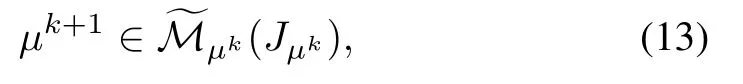
The multiagent rollout ideas that we have discussed so far can be modified and generalized to apply to infinite horizon problems. In this context, we may also consider multiagent versions of PI algorithms, which generate a sequence of policies {µk}. They can be viewed as repeated applications of multiagent rollout, with each policy µkin the sequence being the multiagent rollout policy that is obtained when the preceding policy µk−1is viewed as the base policy.For challenging problems, PI must be implemented off-line and with approximations, possibly involving neural networks.However,the final policy obtained off-line by PI(or its neural network representation) can be used as the base policy for an on-line multiagent rollout scheme.

We will focus on discounted problems with finite number of states and controls, so that the problem has a contractive structure(i.e.,the Bellman operator is a contraction mapping),and the strongest version of the available theory applies(the solution of Bellman’s equation is unique, and strong convergence results hold for PI); see [13], Chapters 1 and 2, [14], Chapter 2, or [2], Chapter 4. However, a qualitatively similar methodology can be applied to undiscounted problems involving a termination state (e.g., stochastic shortest path problems, see [65], Chapter 2, [13], Chapter 3, and [14],Chapters 3 and 4).

In particular, we consider a standard Markovian decision problem (MDP for short) infinite horizon discounted version of the finite horizon m-agent problem of Section I-B, where m>1. We assume n states x=1,...,n and a control u that consists of m components uℓ, ℓ=1,...,m,

u=(u1,...,um),

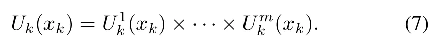
(for the MDP notation adopted for this section, we switch for convenience to subscript indexing for agents and control components, and reserve superscript indexing for policy iterates). At state x and stage k, a control u is applied, and the system moves to a next state y with given transition probability pxy(y)and cost g(x,u,y).When at stage k,the transition cost is discounted by αk, where α ∈(0,1) is the discount factor.Each control component uℓis separately constrained to lie in a given finite set Uℓ(x) when the system is at state x. Thus the control constraint is u ∈U(x), where U(x) is the finite Cartesian product set

U(x)=U1(x)×···×Um(x).

The cost function of a stationary policy µ that applies controlµ(x)∈U(x) at state x is denoted by Jµ(x), and the optimal cost [the minimum over µ of Jµ(x)] is denoted J∗(x).

An equivalent version of the problem, involving a reformulated/expanded state space is depicted in Fig.6 for the case m=3. The state space of the reformulated problem consists of

where x ranges over the original state space (i.e., x ∈{1,...,n}), and each uℓ, ℓ = 1,...,m, ranges over the corresponding constraint set Uℓ(x). At each stage, the agents choose their controls sequentially in a fixed order: from state x agent 1 applies u1∈U1(x) to go to state (x,u1),then agent 2 applies u2∈U2(x) to go to state (x,u1,u2),and so on, until finally at state (x,u1,...,um−1), agent m applies um∈Um(x), completing the choice of control u = (u1,...,um), and effecting the transition to state y at a cost g(x,u,y), appropriately discounted.

This reformulation involves the type of tradeoff between control space complexity and state space complexity that was proposed in the book[65],Section 6.1.4,and was discussed in Section II-C.The reformulated problem involves m cost-to-go functions

J0(x),J1(x,u1),...,Jm−1(x,u1,...,um−1),

with corresponding sets of Bellman equations, but a much smaller control space.Note that the existing analysis of rollout algorithms, including implementations, variations, and error bounds, applies to the reformulated problem; see Section 5.1 of the author’s RL textbook [2]. Moreover, the reformulated problem may prove useful in other contexts where the size of the control space is a concern,such as for example Q-learning.Similar to the finite horizon case, our implementation of the rollout algorithm,which is described next,involves one-agentat-a-time policy improvement,while maintaining the basic cost improvement and error bound properties of rollout,since these apply to the reformulated problem.

Fig.6. Illustration of how to transform an m-agent infinite horizon problem into a stationary infinite horizon problem with fewer control choices available at each state (in this figure m = 3). At the typical stage only one agent selects a control. For example, at state x, the first agent chooses u1 at no cost leading to state (x,u1). Then the second agent applies u2 at no cost leading to state (x,u1,u2). Finally, the third agent applies u3 leading to some state y at cost g(x,u,y), where u is the combined control of the three agents, u = (u1,u2,u3). The figure shows the first three transitions of the trajectories that start from the states x, (x,u1), and (x,u1,u2), respectively. Note that the state space of the transformed problem is well suited for the use of state space partitioned PI algorithms; cf. the book [3], and the papers [10]−[12], [15].

A. Multiagent Rollout Policy Iteration

The policies generated by the standard PI algorithm for the reformulated problem of Fig.6 are defined over the larger space and have the form

We may consider a standard PI algorithm that generates a sequence of policies of the preceding form (see Section IVE), and which based on standard discounted MDP results,converges to an optimal policy for the reformulated problem,which in turn yields an optimal policy for the original problem.However, policies of the form (12) can also be represented in the simpler form

µ1(x),µ2(x),...,µm(x)

i.e., as policies for the original infinite horizon problem. This motivates us to consider an alternative multiagent PI algorithm that uses one-agent-at-a-time policy improvement and operates over the latter class of policies.We will see that this algorithm converges to an agent-by-agent optimal policy(which need not be an optimal policy for the original problem).By contrast,the alternative multiagent PI algorithm of Section IV-E also uses one-agent-at-a-time policy improvement,but operates over the class of policies (12), and converges to an optimal policy for the original problem (rather than just an agent-by-agent optimal policy).

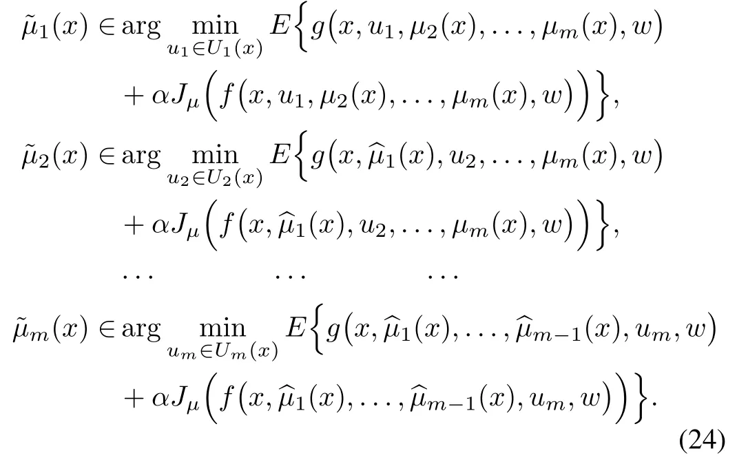
Consistent with the multiagent rollout algorithm of Section IV-D, we introduce a one-agent-at-a-time PI algorithm that uses a modified form of policy improvement, whereby the control u = (u1,...,um) is optimized one-component-at-atime, with the preceding components computed according to the improved policy,and the subsequent components computed according to the current policy.In particular,given the current policy µk, the next policy is obtained as

satisfying for all states x=1,...,n,

Each of the m minimizations (14) can be performed for each state x independently, i.e., the computations for state x do not depend on the computations for other states, thus allowing the use of parallel computation over the different states. On the other hand, the computations corresponding to individual agent components must be performed in sequence(in the absence of special structure related to coupling of the control components through the transition probabilities and the cost per stage). It will also be clear from the subsequent analysis that for convergence purposes, the ordering of the components is not important, and it may change from one policy improvement operation to the next. In fact there are versions of the algorithm,which aim to optimize over multiple component orders, and are amenable to parallelization as discussed in Section II-E.

By contrast, since the number of elements in the constraint set U(x) is bounded by qm, the corresponding number of Qfactor calculations in the standard policy improvement operation is bounded by qm.Thus in the one-agent-at-a-time policy improvement the number of Q-factors grows linearly with m,as compared to the standard policy improvement, where the number of Q-factor calculations grows exponentially with m.

B. Multipass Multiagent Policy Improvement

In trying to understand why multiagent rollout of the form(13)succeeds in improving the performance of the base policy,it is useful to think of the multiagent policy improvement operation as an approximation of the standard policy improvement operation. We basically approximate the joint minimization over all the control components u1,...,umwith a single“coordinate descent-type” iteration, i.e., a round of single control component minimizations, each taking into account the results of the earlier minimizations.

Mathematically, this amounts to using the control components at x of a policy within the set

Similarly, we may consider k >2 rounds of coordinate descent iterations.This amounts to using the control components at x of a policy within the set

will converge (since the control space is finite). However, the limit of these values need not be the result of the joint control component minimization9Generally, the convergence of the coordinate descent method to the minimum of a multivariable optimization cannot be guaranteed except under special conditions, which are not necessarily satisfied within our context.

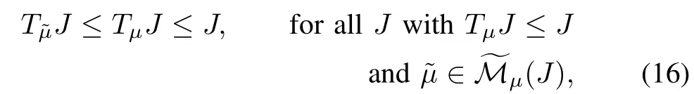
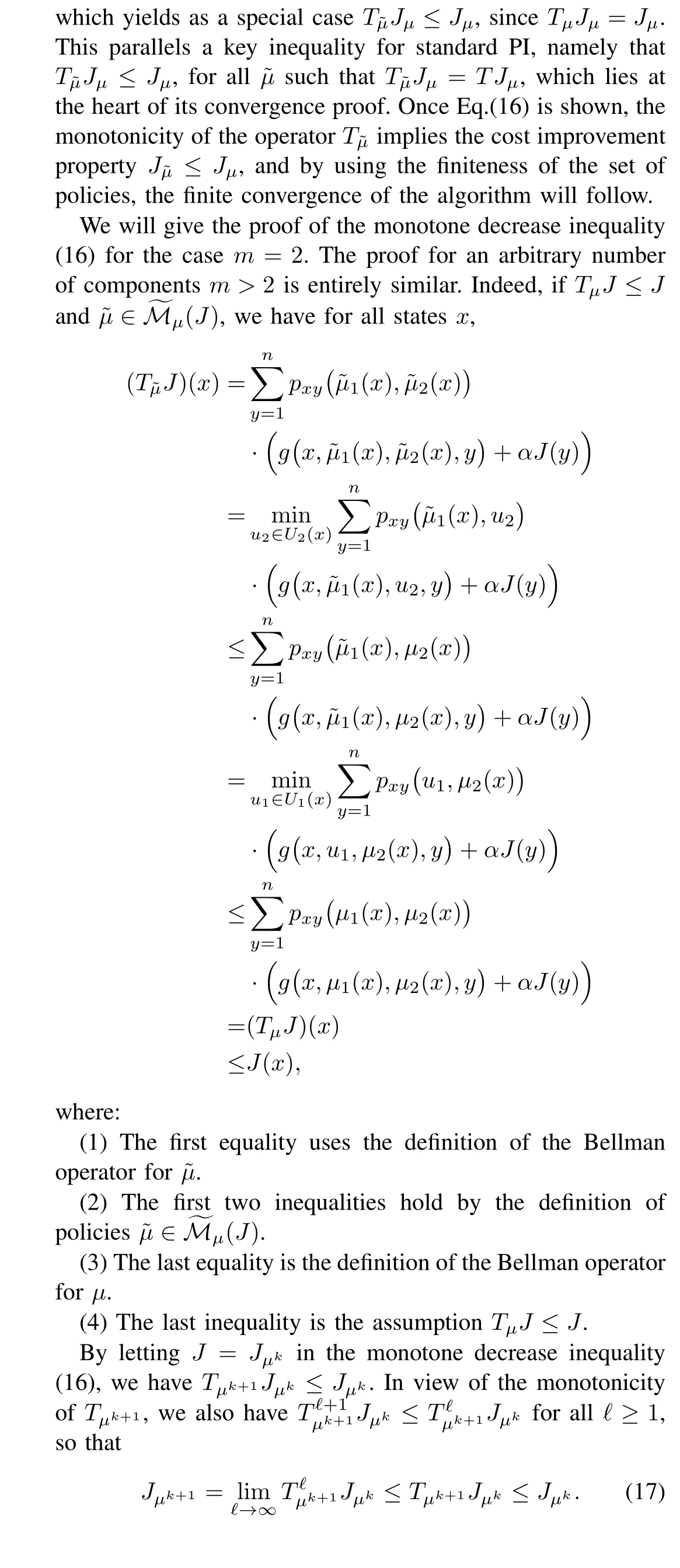
C. Convergence to an Agent-by-Agent Optimal Policy

An important fact is that multiagent PI need not converge to an optimal policy. Instead we will show convergence to a different type of optimal policy, which we will now define.

While an(overall)optimal policy is agent-by-agent optimal,the reverse is not true as the following example shows.

Example 5 (Counterexample for Agent-by-Agent Optimality)

The preceding example is representative of an entire class of DP problems where an agent-by-agent optimal policy is not overall optimal. Any static (single step) multivariable optimization problem where there are nonoptimal solutions that cannot be improved upon by a round of coordinate descent operations(sequential component minimizations,onecomponent-at-a-time)can be turned into an infinite horizon DP example where these nonoptimal solutions define agent-byagent optimal policies that are not overall optimal.Conversely,one may search for problem classes where an agent-by-agent optimal policy is guaranteed to be(overall)optimal among the type of multivariable optimization problems where coordinate descent is guaranteed to converge to an optimal solution.For example positive definite quadratic problems or problems involving differentiable strictly convex functions (see [67],Section 3.7). Generally, agent-by-agent optimality may be viewed as an acceptable form of optimality for many types of problems, but there are exceptions.

Our main result is that the one-agent-at-a-time PI algorithm generates a sequence of policies that converges in a finite number of iterations to a policy that is agent-by-agent optimal.However, we will show that even if the final policy produced by one-agent-at-a-time PI is not optimal,each generated policy is no worse than its predecessor.In the presence of approximations, which are necessary for large problems, it appears that the policies produced by multiagent PI are often of sufficient quality for practical purposes,and not substantially worse than the ones produced by (far more computationally intensive)approximate PI methods that are based on all-agents-at-once lookahead minimization.

For the proof of our convergence result,we will use a special rule for breaking ties in the policy improvement operation in favor of the current policy component. This rule is easy to enforce, and guarantees that the algorithm cannot cycle between policies. Without this tie-breaking rule,the following proof shows that while the generated policies may cycle, the corresponding cost function values converge to a cost function value of some agent-by-agent optimal policy.

In the following proof and later all vector inequalities are meant to be componentwise, i.e., for any two vectors J and J′, we write

J ≤J′ifJ(x)≤J′(x) for all x.

For notational convenience, we also introduce the Bellman operator Tµthat maps a function of the state J to the function of the state TµJ given by

Proposition 2: Let {µk} be a sequence generated by the oneagent-at-a-time PI algorithm (13) assuming that ties in the policy improvement operation of Eq.(14) are broken as follows: If for any ℓ=1,...,m and x,the control componentµℓ(x)attains the minimum in Eq.(14), we choose

[even if there are other control components within Uℓ(x) that attain the minimum in addition to µℓ(x)]. Then for all x and k,we have

and after a finite number of iterations, we have µk+1= µk, in which case the policies µk+1and µkare agent-by-agent optimal.

D. Variants - Value and Policy Approximations

An important variant of multiagent PI is an optimistic version, whereby policy evaluation is performed by using a finite number of one-agent-at-a-time value iterations.This type of method together with a theoretical convergence analysis of multiagent value iteration is given in the paper [5] and in the monograph [3] (Sections 5.4−5.6). It is outside the scope of this paper.

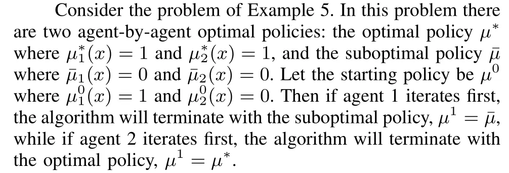
As Example 5 shows,there may be multiple agent-by-agent optimal policies, with different cost functions. This illustrates that the policy obtained by the multiagent PI algorithm may depend on the starting policy. It turns out that the same example can be used to show that the policy obtained by the algorithm depends also on the order in which the agents select their controls.

Example 6 (Dependence of the Final Policy on the Agent Iteration Order)

As noted in Section II-E, it is possible to try to optimize the agent order at each iteration. In particular, first optimize over all single agent Q-factors,by solving the m minimization problems that correspond to each of the agents ℓ = 1,...,m being first in the multiagent rollout order. If ℓ1is the agent that produces the minimal Q-factor, we fix ℓ1to be the first agent in the multiagent rollout order. Then we optimize over all single agent Q-factors, by solving the m −1 minimization problems that correspond to each of the agents ℓ ̸= ℓ1being second in the multiagent rollout order, etc.

1) Value and Policy Neural Network Approximations

The RL books [2] and [3] provide a lot of details relating to the structure and the training of value and policy networks in various contexts, some of which apply to the algorithms of the present paper. These include the use of distributed asynchronous algorithms that are based on partitioning of the state space and training different networks on different sets of the state space partition; see also the paper [15], which applies partitioning to the solution of a challenging class of partial state information problems.

2) Value and Policy Approximations with Aggregation

One of the possibilities for value and policy approximations in multiagent rollout arises in the context of aggregation; see the books [13] and [2], and the references quoted there. In particular, let us consider the aggregation with representative features framework of [2], Section 6.2 (see also [13], Section 6.5).The construction of the features may be done with sophisticated methods, including the use of a deep neural network as discussed in the paper [80]. Briefly, in this framework we introduce an expanded DP problem involving a finite number of additional states i = 1,...,s, called aggregate states. Each aggregate state i is associated with a subset Xiof the system’s state space X. We assume that the sets Xi,i = 1,...,s, are nonempty and disjoint, and collectively include every state of X. We also introduce aggregation probabilities mapping an aggregate state i to the subset Xi,and disaggregation probabilities ϕyjmapping system states y to subsets of aggregate states Xj.

A base policyµdefines a set of aggregate state costs rµ(j),j =1,...,s, which can be computed by simulation involving an “aggregate” Markov chain (see [2], [13]). The aggregate costs rµ(j) define an approximation ˆJµof the cost function Jµof the base policy, through the equation

Note that using an approximation architecture based on aggregation has a significant advantage over a neural network architecture because aggregation induces a DP structure that facilitates PI convergence and improves associated error bounds (see [2] and [13]). In particular, a multiagent PI algorithm based on aggregation admits a convergence result like the one of Prop.2,except that this result asserts convergence to an agent-by-agent optimal policy for the associated aggregate problem. By contrast, approximate multiagent PI with value and policy networks (cf. Fig.7) generically oscillates, as shown in sources such as [2], [13], [65], [81].

E. Policy Iteration and Q-Learning for the Reformulated Problem

Let us return to the equivalent reformulated problem introduced at the beginning of Section IV and illustrated in Fig.6.Instead of applying approximate multiagent PI to generate a sequence of multiagent policies

Fig.7. Approximate multiagent PI with value and policy networks. The value network provides a trained approximation to the current base policy µ. The policy network provides a trained approximation to the corresponding multiagent rollout policy ˜µ. The policy network may consist of m separately trained policy networks, one for each of the agent policies ,...,.

as described in Section IV-A [cf. Eqs.(13) and (14)], we can use an ordinary type of PI method for the reformulated problem.The policies generated by this type of PI will exhibit not only a dependence on the state x [like the policies(19)], but also a dependence on the agents’ controls, i.e., the generated policies will have the form

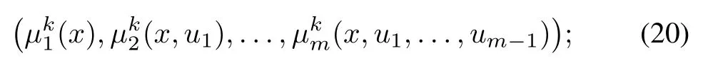
cf. the state space of Eq.(11) of the reformulated problem.Thus the policies are defined over a space that grows exponentially with the number of agents.This is a different PI method than the one of Section IV-A, and will generate a different sequence of policies, even when the initial policy is the same.

The exact form of this PI algorithm starts iteration k with a policy of the form(20),computes its corresponding evaluation(i.e.,the cost function of the policy,defined over the state space of the reformulated problem)

and generates the new policy

According to the standard theory of discounted MDP, the preceding exact form of PI will terminate in a finite number of iterations with an optimal policy

For example, the reader can verify that the algorithm will find the optimal policy of the one-state/two controls problem of Example 5 in two iterations, when started with the strictly suboptimal agent-by-agent optimal policy µ1(x) = 0,µ2(x,u1)≡0 of that problem.

Note that the policy improvement operation (22) requires optimization over single control components rather over the entire vector u=(u1,...,um),but it is executed over a larger and more complex state space,whose size grows exponentially with the number of agents m.The difficulty with the large state space can be mitigated through approximate implementation with policy networks,but for this it is necessary to construct m policy networks at each iteration, with the ℓth agent network having as input (x,u1,...,uℓ−1); cf. Eq.(20). Similarly, in the case of approximate implementation with value networks,it is necessary to construct m value networks at each iteration,with the ℓth agent network having as input (x,u1,...,uℓ−1);cf.Eq.(21).Thus generating policies of the form(20)requires more complex value and policy network approximations. For a moderate number of agents, however, such approximations may be implementable without overwhelming difficulty,while maintaining the advantage of computationally tractable oneagent-at-a-time policy improvement operations of the form(22).

We may also note that the policy improvement operations(22) can be executed in parallel for all states of the reformulated problem. Moreover, the corresponding PI method has a potentially significant advantage: it aims to approximate an optimal policy rather than one that is merely agent-by-agent optimal.

1) Q-Learning for the Reformulated Problem

The preceding discussion assumes that the base policy for the multiagent rollout algorithm is a policy generated through an off-line exact or approximate PI algorithm.We may also use the reformulated problem to generate a base policy through an off-line exact or approximate value iteration(VI)or Q-learning algorithm.In particular,the exact form of the VI algorithm can be written in terms of multiple Q-factors as follows:

Note that all of the iterations(23)involve minimization over a single agent control component,but are executed over a state space that grows exponentially with the number of agents.On the other hand one may use approximate versions of the VI and Q-learning iterations (23) (such as SARSA [78], and DQN [83]) to mitigate the complexity of the large state space through the use of neural networks or other approximation architectures.Once an approximate policy is obtained through a neural network-based variant of the preceding algorithm, it can be used as a base policy for on-line multiagent rollout that involves single agent component minimizations.

F. Truncated Multiagent Rollout and Error Bound

Another approximation possibility, which may also be combined with value and policy network approximations is truncated rollout, which operates similar to the finite horizon case described in Section II-E. Here, we use multiagent onestep lookahead,we then apply rollout with base policyµfor a limited number of steps,and finally we approximate the cost of the remaining steps using some terminal cost function approximation J.In truncated rollout schemes,J may be heuristically chosen, may be based on problem approximation, or may be based on a more systematic simulation methodology. For example, the values Jµ(x) can be computed by simulation for all x in a subset of representative states, and J can be selected from a parametric class of functions through training,e.g., a least squares regression of the computed values. This approximation may be performed off-line, outside the timesensitive restrictions of a real-time implementation, and the result may be used on-line in place of Jµas a terminal cost function approximation.

We have the following performance bounds the proofs of which are given in [3] (Prop. 5.2.7).

These error bounds provide some guidance for the implementation of truncated rollout, as discussed in Section 5.2.6 of the book [3]. An important point is that the error bounds do not depend on the number of agents m, so the preceding proposition guarantees the same level of improvement of the rollout policy over the base policy for one-agent-at-a-time and all-agents-at-once rollout. In fact there is no known error bound that is better for standard rollout than for multiagent rollout. This provides substantial analytical support for the multiagent rollout approach, and is consistent with the results of computational experimentation available so far.

V. AUTONOMOUS MULTIAGENT ROLLOUT FOR INFINITE HORIZON PROBLEMS-SIGNALING POLICIES

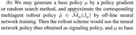
(a) We may use the approximate multiagent PI algorithm with policy network approximation (cf. Section IV-D), start with some initial policy µ0, and produce k new policiesµ1,...,µk.Then the rollout scheme would useµkas signaling policy, and µk−1as base policy. The final rollout policy thus obtained can be implemented on-line with the possibility of on-line replanning and the attendant robustness property.

Example 7 (Autonomous Spiders and Flies)

Let us return to the two-spiders-and-two-flies problem of Examples 2 and 4, and use it as a test of the sensitivity of autonomous multiagent rollout algorithm with respect to variations in the signaling policy. Formally, we view the problem as an infinite horizon MDP of the stochastic shortest path type.Recall that the base policy moves each spider selfishly towards the closest surviving fly with no coordination with the other spider,while both the standard and the multiagent rollout algorithms are optimal.

On the other hand, we saw in Example 4 that if we use as signaling policy the base policy,and the two spiders start at the same position,the spiders cannot coordinate their move choices,and they never separate. Thus the algorithm gets locked onto an oscillation where the spiders keep moving together back and forth, and (in contrast with the base policy) never capture the flies!

The preceding example shows how a misguided choice of signaling policy (namely the base policy), may lead to very poor performance starting from some initial states, but also a very good performance starting from other initial states.Since detecting the “bad” initial states may be tricky for a complicated problem, it seems that one should be careful to support with analysis (to the extent possible), as well as substantial experimentation the choice of a signaling policy.

The example also illustrates a situation where approximation errors in the calculation of the signaling policy matter little. This is the case where at the current state the agents are sufficiently decoupled so that there is a dominant Q-factor in the minimization (24) whose dominance is not affected much by the choice of the signaling policy. As noted in Section III, one may exploit this type of structure by dividing the agents in “coupled” groups, and require coordination of the rollout control selections only within each group, while the computation within different groups may proceed in parallel with a signaling policy such as the base policy. Then the computation time/overhead for selecting rollout controls oneagent-at-a-time using on-line simulation will be proportional to the size of the largest group rather than proportional to the number of agents.11The concept of weakly coupled subsystems figures prominently in the literature of decentralized control of systems with continuous state and control spaces, where it is usually associated with a (nearly) block diagonal structure of the Hessian matrix of a policy’s Q-factors (viewed as functions of the agent control components u1,...,um for a given state). In this context, the blocks of the Hessian matrix correspond to the coupled groups of agents.This analogy, while valid at some conceptual level, does not fully apply to our problem, since we have assumed a discrete control space.Note, however, that the “coupled”groups may depend on the current state, and that deciding which agents to include within each group may not be easy.

Analysis that quantifies the sensitivity of the performance of the autonomous multiagent rollout policy with respect to problem structure is an interesting direction for further research. The importance of such an analysis is magnified by the significant implementation advantages of autonomous versus nonautonomous rollout schemes: the agents can compute on-line their respective controls asynchronously and in parallel without explicit inter-agent coordination, while taking advantage of local information for on-line replanning.

VI. CONCLUDING REMARKS

We have shown that in the context of multiagent problems,an agent-by-agent version of the rollout algorithm has greatly reduced computational requirements, while still maintaining the fundamental cost improvement property of the standard rollout algorithm. There are several variations of rollout algorithms for multiagent problems, which deserve attention.Moreover, additional computational tests in some practical multiagent settings will be helpful in comparatively evaluating some of these variations.

We have primarily focused on the cost improvement property, and the important fact that it can be achieved at a much reduced computational cost. The fact that multiagent rollout cannot improve strictly over a (possibly suboptimal)policy that is agent-by-agent optimal is a theoretical limitation,which, however, for many problems does not seem to prevent the method from performing comparably to the far more computationally expensive standard rollout algorithm (which is in fact intractable for only a modest number of agents).

It is useful to keep in mind that the multiagent rollout policy is essentially the standard (all-agents-at-once) rollout policy applied to the (equivalent) reformulated problem of Fig.3 (or Fig.6 in the infinite horizon case).As a result,known insights,results, error bounds, and approximation techniques for standard rollout apply in suitably reformulated form.Moreover,the reformulated problem may form the basis for an approximate PI algorithm with agent-by-agent policy improvement, as we have discussed in Section IV-E.

In this paper, we have assumed that the control constraint set is finite in order to argue about the computational efficiency of the agent-by-agent rollout algorithm. The rollout algorithm itself and its cost improvement property are valid even in the case where the control constraint set is infinite, including the model predictive control context (cf. Section II-E of the RL book [2]), and linear-quadratic problems. However, it is as yet unclear whether agent-by-agent rollout offers an advantage in the infinite control space case, especially if the one-step lookahead minimization in the policy improvement operation is not done by discretization of the control constraint set, and exhaustive enumeration and comparison of the associated Qfactors.

The two multiagent PI algorithms that we have proposed in Sections IV-A and IV-E differ in their convergence guarantees when implemented exactly. In particular the PI algorithm of Section IV-A,in its exact form,is only guaranteed to terminate with an agent-by-agent optimal policy. Still in many cases(including the problems that we have tested computationally)it may produce comparable performance to the standard PI algorithm,which however involves prohibitively large computation even for a moderate number of agents. The PI algorithm of Section IV-E,in its exact form,is guaranteed to terminate with an optimal policy, but its implementation must be carried out over a more complex space. Its approximate form with policy networks has not been tested on challenging problems, and it is unclear whether and under what circumstances it offers a tangible performance advantage over approximate forms of the PI algorithm of Section IV-A.

Our multiagent PI convergence result of Prop.2 can be extended beyond the finite-state discounted problem to more general infinite horizon DP contexts,where the PI algorithm is well-suited for algorithmic solution. Other extensions include agent-by-agent variants of value iteration, optimistic PI, Qlearning and other related methods. The analysis of such extensions is reported separately; see [3] and [5].

We have also proposed new autonomous multiagent rollout schemes for both finite and infinite horizon problems. The idea is to use a precomputed signaling policy,which embodies sufficient agent coordination to obviate the need for interagent communication during the on-line implementation of the algorithm. In this way the agents may apply their control components asynchronously and in parallel. We have still assumed,however, that the agents share perfect state information (or perfect belief state information in the context of partial state observation problems).Intuitively,for many problems it should be possible to implement effective autonomous multiagent rollout schemes that use state estimates in place of exact states. Analysis and computational experimentation with such schemes should be very useful and may lead to improved understanding of their properties.

Several unresolved questions remain regarding algorithmic variations and conditions that guarantee that our PI algorithm of Section IV-A obtains an optimal policy rather than one that is agent-by-agent optimal (the paper [5] provides relevant discussions). Moreover, approximate versions of our PI algorithms that use value and policy network approximations are of great practical interest,and are a subject for further investigation(the papers by Bhattacharya et al.[15]and[64]discuss in detail various neural network-based implementations, in the context of some challenging POMDP multi-robot repair applications). Finally, the basic idea of our approach, namely simplifying the one-step lookahead minimization defining the Bellman operator while maintaining some form of cost improvement or convergence guarantee,can be extended in other directions to address special problem types that involve multicomponent control structures.

We finally mention that the idea of agent-by-agent rollout also applies within the context of challenging deterministic discrete/combinatorial optimization problems, which involve constraints that couple the controls of different stages. While we have not touched upon this subject in the present paper,we have discussed the corresponding constrained multiagent rollout algorithms separately in the book[3]and the paper[6].