
CONSTRUCTION OF IMPROVED BRANCHING LATIN HYPERCUBE DESIGNS∗
2021-09-06 07:54陈浩
关键词:陈浩
(陈浩)
School of Statistics,Tianjin University of Finance and Economics,Tianjin 300222,China E-mail:chlh1985@126.com
Jinyu YANG (杨金语) Min-Qian LIU (刘民千)†
School of Statistics and Data Science,LPMC&KLMDASR,Nankai University,Tianjin 300071,China E-mail:jyyang@nankai.edu.cn;mqliu@nankai.edu.cn
Abstract In this paper,we propose a new method,called the level-collapsing method,to construct branching Latin hypercube designs(BLHDs).The obtained design has a sliced structure in the third part,that is,the part for the shared factors,which is desirable for the qualitative branching factors.The construction method is easy to implement,and(near)orthogonality can be achieved in the obtained BLHDs.A simulation example is provided to illustrate the effectiveness of the new designs.
Key words Branching and nested factors;computer experiment;Gaussian process model;orthogonality
1 Introduction
Many experiments involve factors that only exist within the levels of another factor.Take printed circuit board(PCB)manufacturing,for example([1]).Here,the surface preparation method is a qualitative factor having two levels:mechanical scrubbing and chemical treatment.Under each of the two levels,there exist two different factors:pressure and micro-etch.More precisely,the factor pressure only exists when the method involves mechanical scrubbing,and micro-etch rate only exists under the level of chemical treatment.Following the de finitions in[1],the factors that only exist within the levels of another factor(like the pressure and the microetch rate)are called nested factors.Accordingly,a factor within which other factors are nested is called a branching factor;these include things such as the surface preparation method for PCB manufacturing.Such experimental situations are often encountered in computer experiments as well,for example,the motivation example of[1].The objective of that example is to optimize a turning process for hardened bearing steel with a cBN cutting tool.There is one branching factor,called the cutting edge shape,which has two levels:chamfer and hone edge.Within the chamfer,two factors(length and angle)are nested,while no factor is nested in the hone edge.In addition,there are six other factors(cutting edge radius,tool nose radius,rake angle,cutting speed,feed and depth of cut),called shared factors,which are common to both the branching and nested factors.
Although experiments with branching and nested factors are commonly encountered,there is little literature on the design construction for such experiments.Taguchi[2]proposed pseudofactor designs by carefully assigning branching and nested factors to the columns of orthogonal arrays(OAs,[3]),where the pseudo-factor is in fact the nested factor.Later,in[4],such designs were called branching designs.However,as stated in[1],Taguchi’s method is not sufficiently general to be applied to computer experiments.Instead,Hung et al.[1]developed branching Latin hypercube designs(BLHDs)to suit computer experiments with branching and nested factors.A BLHD consists of three parts:(i)an OA for the branching factors;(ii)several Latin hypercube designs(LHDs)([5])for the nested factors;(iii)an LHD for the shared factors.An example of a BLHD is given in Table 1(Table 3 in[1]);here the BLHD has eight runs,one branching factorz
,one nested factorv
,and two shared factors:x
andx
.As pointed out in[1],the same levels ofv
(for example two 1’s)do not have the same meaning.Such a frame of a BLHD looks attractive,however the third part has no sliced structure to accommodate the qualitative branching factor.The superiority of sliced Latin hypercube designs(SLHDs)over ordinary LHDs was proved by both theoretical and simulated results in[6]when being used for computer experiments with both qualitative and quantitative factors.Thus an SLHD is more effective as the third part of a BLHD than an LHD.For an SLHD,not only the whole design,but also its slices achieve the maximum strati fication in any one-dimensional projection.Such a good property ensures that when the third part is collapsed onto the branching factor,each factor in the third part gets maximum strati fication under each level of the branching factor.Take the design in Table 1 as an example;when the third part is collapsed ontoz
,it becomes the following matrix: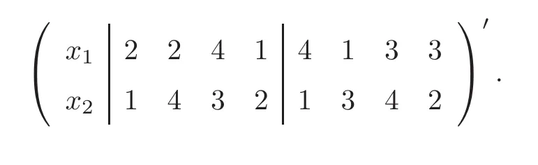

Table 1 An example of a BLHD
It is easy to see that the first columnx
does not get the maximum strati fication under either level ofz
,which can be seen more clearly from the scatter plot in Figure 1(a);that is,when considering the projection onx
,there are two points falling into either of the intervals[1/
4,
2/
4)and[2/
4,
3/
4).Note that the levels ofx
andx
in Figure 1 are mapped into[0,
1)through(x
−0.
5)/
8,wherex
is thei
th level of factorx
fori
=1,...,
8 andj
=1,
2.However,if we exchange the second and seventh elements ofx
in Table 1,then the third part becomes an SLHD with 8 runs,2 factors and 2 slices.Now,the collapsed matrix becomes
Figure 1 (a)Scatter plot of the third part of the BLHD in Table 1;(b)Scatter plot of the third part obtained by exchanging the 2nd and 7th elements of x1in Table 1.The symbols ‘◦’and ‘+’represent the four runs from the first and second slices,respectively.

,
1/
4),
[1/
4,
2/
4),
[2/
4,
3/
4),
[3/
4,
1)in each dimension;that is,each slice gets the maximum strati fication in any 4×1 or 1×4 grid.In this paper,we focus on introducing a sliced structure into the third part of BLHDs,and propose a levelcollapsing method to construct BLHDs.The obtained designs,referred to as improved BLHDs(IBLHDs),have a better structure than existing BLHDs,and can achieve near orthogonality more easily.The remainder of this paper is organized as follows:Section 2 provides the level-collapsing method for constructing IBLHDs.Section 3 discusses the(near)orthogonality of the IBLHDs.An example for illustrating their effectiveness is presented in Section 4.Section 5 contains some concluding remarks.
2 Construction of IBLHDs
First,we give some de finitions and notation.For any real numberr
,「r
⏋denotes the smallest integer greater than or equal tor
,and for a real vector or matrixM
,「M
⏋is de fined to its elements.A permutation onZ
is a rearrangement of 1,...,n
,and alln
!rearrangements are equally probable.Ann
×q
matrix is called a Latin hypercube design(LHD),denoted byL
(n,q
),if each column is a permutation onZ
,and these columns are obtained independently.Denote an SLHD withn
runs,q
factors ands
slices bySL
(n,q,s
).Next,we propose the level-collapsing method for constructing IBLHDs.Without loss of generality,assume that there is only one branching factor,z
,withs
levels,under each of which anL
(n
,m
)is nested.In addition,t
shared factors are involved.Algorithm 2.1
Step 1
Letz
=(1,...,
1,...,s,...,s
)be the branching factor,where each leveli
appearsn
times fori
=1,...,s
.Step 2
Construct anSL
(sn
,m
+t,s
)by the method in[6],denoted byS
=(S
,S
),whereS
includesm
columns ofS
,andS
includes the leftt
columns.
SL
(n,t,s
)instead of anL
(n,t
),which guarantees that each shared factor gets the maximum strati fication under each level of the branching factor;(ii)the LHDs in the second part are obtained by collapsing some columns of the SLHDs constructed in Step 2,which makes it easier to develop(near)orthogonality between factors.
Table 2 IBLHD with one branching factor

Table 3 IBLHD in Example 3.3

Table 4 Correlations among v1,v2,x1and x2
Remark 2.2
Note that for a BLHD,it may happen that there is no nested factor under some level of the branching factor([1]).In this case,we just need to delete the corresponding LHD in the second part of an IBLHD.3 Nearly Orthogonal IBLHDs
Orthogonality is a desirable property for experimental designs,because it guarantees that the main effects can be estimated uncorrelatedly under the first-order polynomial model.In this section,we consider nearly orthogonal IBLHDs,in which nested factors are orthogonal to each other,orthogonal to the shared factors for the whole IBLHD,and nearly orthogonal to the shared factors within each slice.
Let us now see some further de finitions.A design is said to be orthogonal if the correlation between any two distinct columns is zero.AnSL
(n,q,s
)is called a sliced orthogonal LHD(SOLHD,[7–12]),denoted bySOL
(n,q,s
),if both the whole design and its slices are orthogonal.From the construction method in Algorithm 2.1,if the original SLHD in Step 2 is an SOLHD,then the obtained IBLHD will inherit the orthogonality to some extent.In this paper,we only take the SOLHDs constructed by Algorithm 1 in[10]as the SLHDs in Step 2 of Algorithm 2.1.Other SOLHDs in the aforementioned literature can also be used of course,and the results will be similar,that is,the resulting IBLHDs are nearly orthogonal.To present the results in Proposition 3.1,we first brie fly introduce Algorithm 1 in[10].

OD
(m
)’s,Yang et al.[10]constructedSOL
(2sm,m,s
)by
D
,...,D
areOD
(m
)’s with(a,b
),...,
(a,b
),respectively,anda
=2s
andb
=−a
+(2j
−1)forj
=1,...,s
.When projected onto each dimension,each of the 2m
equally spaced intervals[−2sm,
−2s
(m
−1)),
[−2s
(m
−1),
−2s
(m
−2)),...,
[−2s,
0),
[0,
2s
),...,
[2s
(m
−1),
2sm
)contains exactly one point of each slice.Proposition 3.1
Without loss of generality,assume that there is only one branching factor withs
levels.If the SLHDS
=(S
,S
)in Step 2 of Algorithm 2.1 is anSOL
(2sm,m,s
)in(3.1),then(i)the nested factors are orthogonal to the shared factors for the whole IBLHD,and nearly orthogonal to the shared factors within each slice,and the upper bound for the absolute correlations between any nested factor and any shared factor in thej
th slice is

(ii)the nested factors are orthogonal to each other for both the whole design and its slices.
Before proving Proposition 3.1,we present an obvious lemma with its proof omitted.
Lemma 3.2
Assume thatD
is anOD
(m
),wherem
=2andr
≥1 is an integer,and letT
=(T
,...,T
)=(D
,
−D
).Then(i)T
is one permutation on set{−ma
−b,
−(m
−1)a
−b,...,
−a
−b,a
+b,...,
(m
−1)a
+b,ma
+b
},j
=1,...,m
;(ii)T
can be collapsed to one permutation on{1,...,
2m
}by linear transformation
T
is thei
th element ofT
,P
=b/a
+m
+1for the negative levels ofT
,andP
=−b/a
+m
for the positive levels ofT
.
m
levels ofA
are negative.Then based on the structure of theSOL
(2sm,m,s
)in(3.1),
C
andB
is
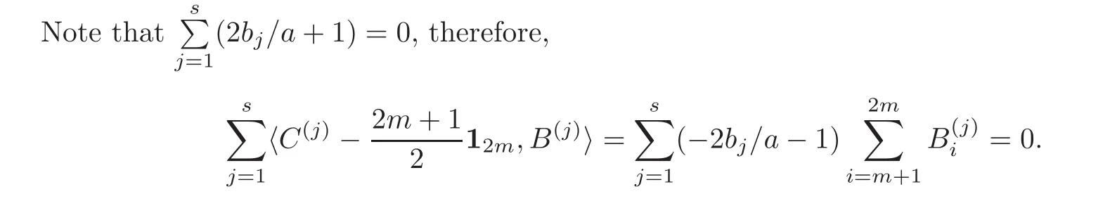
Thus,the nested factors are orthogonal to the shared factors for the whole IBLHD.This completes the proof of(i).
(ii)Denote the columns of any two nested factors in thej
th slice of the IBLHD byC
andC
,respectively,which are collapsed fromA
andA
by linear transformation based on(3.3),j
=1,...,s
.Note that 〈A
,A
〉=0,and thus,
C
,C
)=0.Therefore,the nested factors are orthogonal to each other within each slice.The orthogonality also holds for the whole design.This completes the proof of(ii).Note that in Proposition 3.1,the nested factors are orthogonal to the shared factors for the whole IBLHD,however,if some other SOLHDs are used as the SLHDs in Step 2 of Algorithm 2.1,the nested factors may only be nearly orthogonal to the shared factors for the whole IBLHD.Usually,the values of(3.2)are small,for example,whenm
=8,s
=3,a
=6,b
=−5,b
=−3,b
=−1.In this case,the upper bounds(3.2)for the three slices are 0.
0162,
0.
0153 and 0.
0431,respectively.An illustrative example is given below.Example 3.3
Consider a computer experiment with 16 runs,one branching factorz
with two levels−1 and+1,two nested factorsv
andv
,and two shared factorsx
andx
.According to Algorithm 2.1 and Proposition 3.1,we take anSOL
(16,
4,
2)from[10]witha
=4,b
=−3,b
=−1,which is
S
,and after they are collapsed overz
,the final IBLHD is presented in Table 3.We can compute the upper bounds given in(3.2),which are 0.
0525 and 0.
0434 for the two slices.The real correlations between the nested factors and shared factors for the two slices and the whole design are listed in Table 4,which verify the conclusions in Proposition 3.1.Moreover,we can see that the upper bounds(3.2)are attainable.4 Effectiveness of IBLHDs
In this section,we mainly study the performance of IBLHDs when they are used for building Gaussian process(GP)models.Although integrated analysis has been proven to be better than independent analysis([14]),we insist on using independent analysis in this paper,because different levels of the branching factor often represent remarkably different things,such as the two surface treatment methods in[1].That is to say,the data under one level of the branching factor is probably irrelevant with the data under another one,therefore,they can borrow no strength from one another to improve the fitted model.

f
(x),...,f
(x))is a vector of pre-speci fied regression functions and β=(β
,...,β
)is a vector of unknown coefficients.The residualε
is assumed to be a stationary GP with zero mean and covariance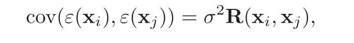
,
x)is the Gaussian correlation function,whose popular form is the product exponential correlation function([15])that will be used in this paper:
θ
,...,θ
)is a vector of scale parameters.Usually,a maximum likelihood method is adopted to estimate the parameters(β,σ
,
θ).Following the normality assumption of the GP model,the log-likelihood function of the collected data is
θ
)is then
×n
correlation matrix with the(i,j
)th element being R(x,
x)and F=(f(x),...,
f(x)).As is stated in[16],simultaneous maximization over(β,σ
,
θ)is unstable because R(θ)may be nearly singular andσ
could be very small.Furthermore,β and θ play different roles:β is used to model overall trend,while θ is a smoothing parameter vector.Thus it is desirable to estimate these things separately.After giving θ,the maximum likelihood estimators(MLE)of β andσ
can be derived from(4.1)as follows: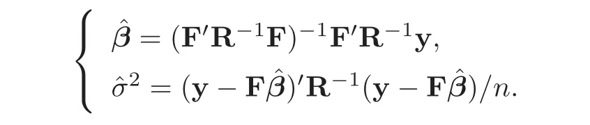
Then the MLE of θ can be obtained as

y
at an untried point xis


Next,we present an illustrative example which was implemented using the Matlab toolbox DACE([17]).
Example 4.1
Assume there is a branching factorz
with two levels,−1 and+1,and under each of these the nested factorv
has eight levels:1,...,
8.In addition,three shared factors,x
,x
andx
,are involved,and sixteen runs are available.The real response function is assumed to be


Figure 2 Boxplots of the 1000 RMSPEs corresponding to BLHDs and IBLHDs.

Table 5 Mean and standard deviation values of RMPSEs in Example 4.1
Note that in this section we fit a separate GP model for each level of the branching factor,otherwise we would need a special kernel function.
5 Concluding Remarks
In this paper,we proposed a new method for constructing BLHDs,and showed that the obtained IBLHDs improve the BLHDs in terms of the projection property under each level of the branching factor;that is,not only the whole design but also the slices get maximum strati fication in one-dimensional projection.In addition,if the original SLHDs are orthogonal,then in the obtained IBLHDs,the nested factors are orthogonal to each other,orthogonal to the shared factors for the whole design,and nearly orthogonal to the shared factors within each slice.Furthermore,the example shows that the IBLHDs outperform the BLHDs when used for building a GP model and for predictions at new points.
Note that all the optimization criteria in[1],including maximin distance,minimum correlation and orthogonal-maximin,can be applied on IBLHDs to get corresponding optimal IBLHDs.Although the nested factors are quantitative in both this paper and[1],they can be qualitative sometimes.Chen et al.[12]constructed SLHDs with both the branching and nested factors being qualitative.In addition,we can also construct the second and third parts of an IBLHD using the OA-based idea([18–20]).
猜你喜欢
Chinese Physics B(2022年8期)2022-08-31
Plasma Science and Technology(2022年7期)2022-08-01
鸭绿江(2021年26期)2021-11-20
娃娃乐园·绘本(2021年9期)2021-09-13
红楼梦学刊(2019年2期)2019-04-12
电子技术与软件工程(2016年24期)2017-02-23
商业文化(2016年16期)2016-09-05
小说月刊(2011年2期)2011-03-15
故事林(2010年3期)2010-05-14
故事林(2010年2期)2010-05-14
 Acta Mathematica Scientia(English Series)2021年4期
- Acta Mathematica Scientia(English Series)的其它文章
- LIMIT CYCLE BIFURCATIONS OF A PLANAR NEAR-INTEGRABLE SYSTEM WITH TWO SMALL PARAMETERS∗
- SLOW MANIFOLD AND PARAMETER ESTIMATION FOR A NONLOCAL FAST-SLOW DYNAMICAL SYSTEM WITH BROWNIAN MOTION∗
- DYNAMICS FOR AN SIR EPIDEMIC MODEL WITH NONLOCAL DIFFUSION AND FREE BOUNDARIES∗
- A STABILITY PROBLEM FOR THE 3D MAGNETOHYDRODYNAMIC EQUATIONS NEAR EQUILIBRIUM∗
- THE GROWTH AND BOREL POINTS OF RANDOM ALGEBROID FUNCTIONS IN THE UNIT DISC∗
- SHOCK DIFFRACTION PROBLEM BY CONVEX CORNERED WEDGES FOR ISOTHERMAL GAS∗