Exciton emission dynamics in single InAs/GaAs quantum dots due to the existence of plasmon-field-induced metastable states in the wetting layer∗

Junhui Huang(黄君辉),Hao Chen(陈昊),Zhiyao Zhuo(卓志瑶),Jian Wang(王健),Shulun Li(李叔伦),Kun Ding(丁琨),Haiqiao Ni(倪海桥),Zhichuan Niu(牛智川),3,Desheng Jiang(江德生),Xiuming Dou(窦秀明),†,and Baoquan Sun(孙宝权),3,‡

1State Key Laboratory of Superlattices and Microstructures,Institute of Semiconductors,Chinese Academy of Sciences,Beijing 100083,China

2College of Materials Science and Optoelectronic Technology,University of Chinese Academy of Sciences,Beijing 100049,China

3Beijing Academy of Quantum Information Sciences,Beijing 100193,China

Keywords:quantum dots,collective excitations,charge carriers,time resolved spectroscopy

1.Introduction

By changing the emitter’s electromagnetic local density of states(LDOS),the spontaneous radiative rate of the emitter will be changed as first pointed out by Purcell.[1]In the vicinity of the metal nanostructures,a modification of LDOS can be realized by confining the incident light within regions far below the diffraction limit to generate modes of localized surface plasmons(LSPs),[2–5]in which the spontaneous recombination rate is enhanced owing to the increase of LDOS.On the other hand,the recombination rate of the emitter was reported to be reduced for an emitter in front of a planar interface,[6]or near metal nanostructures.[7]This phenomenon is related to the destructive interference of the dipole fields between the emitters and reflected field,which results in a decrease of LDOS at the site of emitters.

In our previous report,a very long lifetime of non-single exponential decay characteristics in InAs/GaAs single quantum dots(QDs)was observed due to the destructive interference of the dipole fields between the emitters(excitons in the wetting layer(WL))and metal islands,which results in a decrease of the LDOS in two-dimensional excitons and the formation of a long-lifetime metastable state in the WL.[7]In fact,a similar long lifetime with non-single exponential decay had been reported in many different systems[8–10]and for interpreting the long lifetime decay characteristics,a model with three-level configuration in which a third lower level of long-lived energy state was proposed.For example,a threelevel charge-separated(CS)dark state model associated with quantum tunnelling was applied successfully.[11]In addition,there were the log-normal distribution model assuming statistical law of rate distribution,[12]and the stretched exponential model caused by hopping-transport[13,14]or trapping[15]of the carriers.

2.Materials and methods

The studied low-density InAs/GaAs QD samples were grown by molecular beam epitaxy(MBE)on a(001)semiinsulating GaAs substrate. The corresponding discrete QD emission lines can be isolated by using confocal microscopy.Details of the sample growth procedure can be found elsewhere.[16,17]The epitaxial growth of InAs/GaAs QD samples consists of a 300 nm GaAs buffer layer,a 100 nm AlAs sacrificial layer,a 20 nm GaAs layer,an InAs WL of about one atomic layer thickness,an InAs QD layer,and a 100 nm GaAs cap layer.After etching away the AlAs sacrificed layer,the QD film of 120 nm was separated and transferred onto a polished metal sheet with random distribution of metal islands.

Photoluminescence(PL)and time-resolved photoluminescence(TRPL)spectra of QDs were performed at 7 K using 640 nm excitation from a pulsed semiconductor laser with a pulse length of 40 ps.For measuring the long-lifetime decay curves,the laser pulse repetition rate was set to 1 MHz.A spot of about 2µm in diameter was focused on the sample using a confocal microscope objective lens(NA,0.55).The PL spectral signal was extracted with the same microscope objective,dispersed by 500 mm focal length monochromator and recorded by silicon charged coupled device(CCD).The TRPL spectra were measured by a time-correlated singlephoton counting(TCSPC)device with a time resolution of 280 ps,and the photon auto-correlation function g(2)(τ)measurements were carried out using the Hanbury-Brown and Twiss(HBT)setup at 7 K using 640 nm excitation from a continuous wave laser.

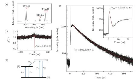
Fig.1.(a)PL spectrum of the positively charged exciton(X+,908.15 nm),exciton(X,911.25 nm)and biexciton emission(XX,912.46 nm).(b)TRPL of the X+emission at an excitation of power of 2.5µW.The red line is a fitting result by using Eq.(9)and obtained average lifetime of〈τ〉=207.6±0.7 ns.Inset:Zoomed in at 0–20 ns of TRPL and linear fitting to the data(red line)with a decay time of 0.93±0.02 ns.(c)g2(t)measurement of the QD emission with continuous wave excitation at an excitation power of 0.043µW.The red line is a fitting result by using Eq.(18).The g2(0)value is obtained as 0.23±0.09.(d)Schematic diagram of three-level model with a long-lived metastable level|3〉and an excited state|2〉as well as the ground state|1〉of the excitons.

3.Results and discussion

The PL spectrum of a single QD excited by pulse laser with a repetition rate of 1 MHz is presented in Fig.1(a),corresponding to the positively charged exciton(X+,908.15 nm),exciton(X,911.25 nm)and biexciton emission(XX,912.46 nm).These emission lines have been identified previously using the polarization-resolved PL spectra.[18,19]The emission intensities are greatly enhanced after the QD sample was transferred onto metal islands and the different excitonic emission lines measured by corresponding PL and TRPL actually show similar characteristics.[7]Here,we will focus on the emission line of X+with the strongest fluorescence intensity to understand the exciton emission dynamics with a long lifetime in detail.The typical TRPL spectrum is presented in Fig.1(b)at the condition of over-saturated excitation power P=2.5µW,showing a fast decay part with a lifetime of approximately 1 ns(see inset of Fig.1(b)),which can be fit by using a single exponential function and a very long lifetime decay of 100 ns order of magnitude.[7]In addition,the corresponding g(2)(τ)results at continuous wave laser excitation exhibits bunching and antibunching characteristics,as shown in Fig.1(c).It is known that the antibunching property is related to a single QD emission,while the bunching property is generally related to the fact that there exists a third long lifetime shelving state.[20]

We note that the long lifetime decay curve cannot be fitted by a single exponential function.Actually,similar nonsingle exponential decays had been reported and interpreted by introducing a third long-lived level below the excited state of emission.[11–13,15]Here it was found that the observed long lifetime decay curve is related to the fact that there exists a metastable state in the WL,which was revealed by lifetime measurements at different excitation wavelengths in our previous work.[7]

Since the energy level of the WL is higher than the excited state level of exciton in the QD,we propose a three-level model,as schematically shown in Fig.1(d),to deduce the exciton decay equations and simulate the unique experimental results.It is shown in Fig.1(d)that the QD emits from the excited state|2〉to the ground state|1〉,and the higher metastable state level|3〉is the level of WL.This is a simplified model of the whole system.In fact,in the experiment,a 640 nm laser is used to excite the GaAs barrier at first and optically pumped electrons and holes will rapidly relax into the WL and QDs.If there is no long lifetime metastable state,excitons in QDs and WL emit PL in a decay time of approximately 1 ns.While if there exists a long lifetime metastable state in the WL,after initial exciton in QDs emits PL which corresponds to the fast decay process,more excitons in the WL will diffuse,be trapped by QDs again and emit fluorescence in QDs,which corresponds to the long lifetime decay process,as the measured TRPL curve representatively shown in Fig.1(b).

Based on the three-level model in Fig.1(d),we can establish a set of rate equation for describing the exciton emission from the QDs and WL after the optical excited electrons and holes relax to and populate the levels of|2〉and|3〉,

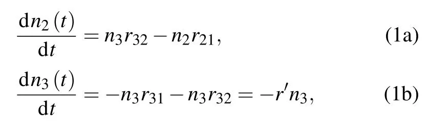
where n2and n3are the population rates of excitons in level|2〉and|3〉,r12and r21the excitation and radiation rates of level|2〉,r13and r31the excitation and radiation rates of|3〉,r32the trapped rate of exciton by QDs,and r′≡r31+r32.Next we will discuss the following two cases:①level|3〉is a normal state with a lifetime of approximately 1 ns and②level|3〉is a long lifetime metastable state.

For case①r32≫r21,r31,Eq.(1a)can be written as

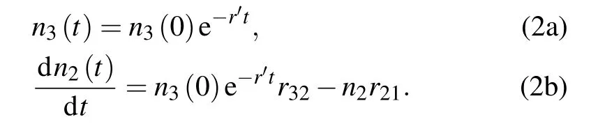
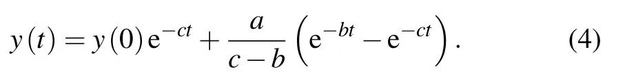
Setting y≡n2(t),a≡n3(0)r32,b≡r′,c≡r21,Eq.(2b)can be rewritten as

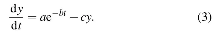
The Laplace transformation is used to solve the above equation,then we get the solution

Thus,the population rate of energy level|2〉is

Since r32≫r21,r31,QD emission intensity I(t)can be expressed as

Thus Eq.(6)can be used to fit the fast decay part of TRPL curve,as shown in the inset of Fig.1(b)by the red line.A lifetime of 1/r21=0.93±0.02 ns is obtained.This result demonstrates that in this approximation the fluorescent decay lifetime of QDs is mainly determined by QD spontaneous radiation decay process.

We consider the fact that the decay time of excitons in level|2〉is approximately 1 ns and it is assumed that r21≫r32,then dn2(t)/dt≈0 compared with the first term of n3r32in Eq.(8).Therefore,the PL intensity as a function of time is mainly determined by the trapping process of excitons,which can be written as

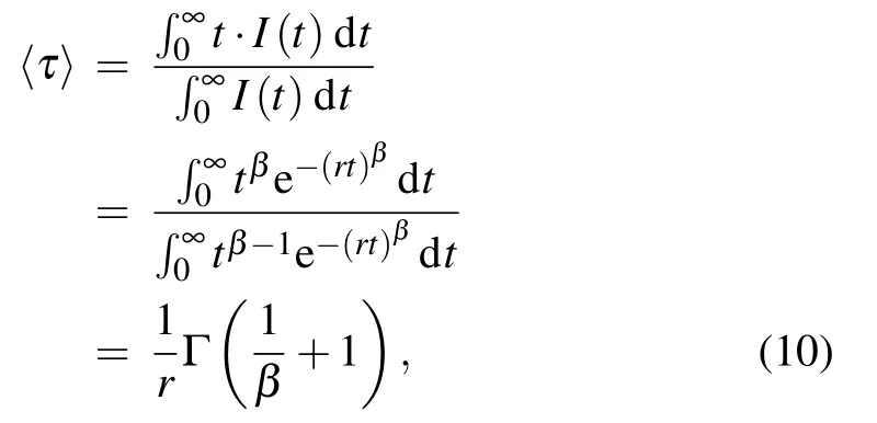
where theΓis the mathematical Gamma function.Therefore,we can use Eq.(9)to fit the TRPL curve,to get the fitting parameters of r andβand calculate the decay time〈τ〉from Eq.(10).The fitting result using Eq.(9),as shown in Fig.1(b)by the red line,gives 1/r=194.4±0.6 ns and β=0.876±0.002.From Eq.(10),the corresponding average decay time〈τ〉=207.6±0.7 ns.

TRPL spectra as a function of excitation power are shown in Figs.2(a)–2(c),where three typical TRPL results under excitation power of P=0.011,0.132 and 1.075µW are exhibited,corresponding to the long lifetime values of〈τ〉=590±20,303±2 and 193.1±0.5 ns,respectively.These values are obtained by fitting the TRPL curves(red lines in Figs.2(a)–2(c))using Eq.(9)and calculating〈τ〉using Eq.(10).The summarized plots of〈τ〉and the stretched factorβas a function of excitation power are shown in Fig.2(d).It is shown that when excitation power increases the lifetime〈τ〉decreases gradually from approximately 750 ns to 200 ns andβchanges from approximately 0.6 to 0.8.Sinceα=1−β,αvalue will become smaller with increasing excitation power.The power dependence can be properly explained with our threelevel model.With the increase of power,more excitons are excited in the wetting layer,and the rate of depletion region formation through capturing of quantum dots decreases,that is,the diffusion rate of depletion region decreases.As the degree of diffusion effect becomes weaker,the attenuation curve tends to be a single exponential as the power increases.The decrease of the lifetime value indicates that the inhibition degree of the average exciton radiation in the wetting layer decreases.This is because the increasing charge background in the wetting layer with the increase of excitation power will act as shielding,thus reducing the inhibition degree and the lifetime decreases with increasing power.

Next we will analyze the measured g(2)(τ)result shown in Fig.1(c),which exhibits bunching and antibunching characteristics.Based on a three-level model(see Fig.1(d)),and assuming that the population rates of excitons in level|1〉,|2〉and|3〉are p1(t),p2(t)and p3(t),respectively,the rate equation in matrix form can be written as

Its solution has the following form:

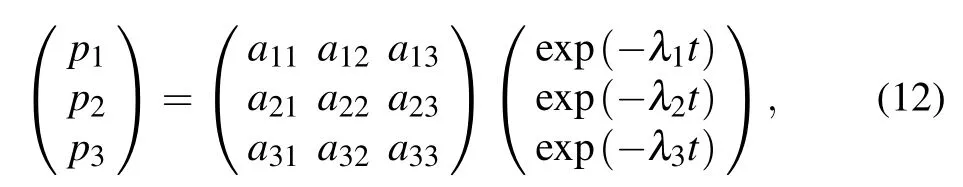
where theλiequals to the eigenvalues of the matrix of Eq.(12),i.e.,

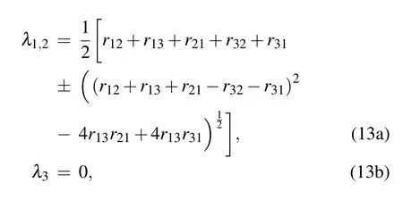
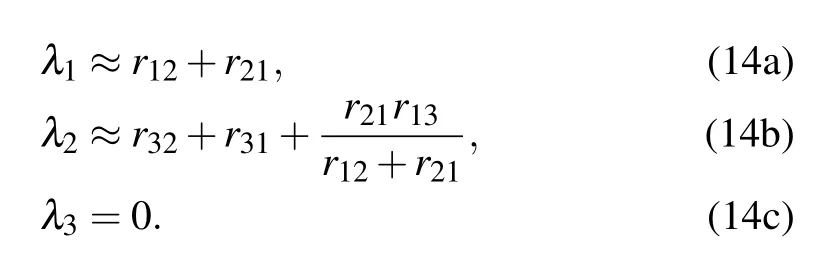
By considering the approximation of low transition rates to and from the metastable state|3〉,r13,r31and r32can be regarded as small quantities andλ1andλ2can be expressed as

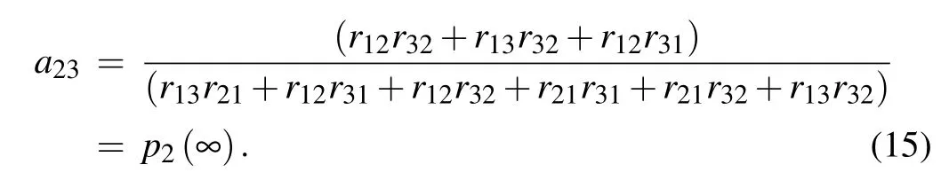
Considering the t→∞limit,in which the system is in equilibrium,we can get

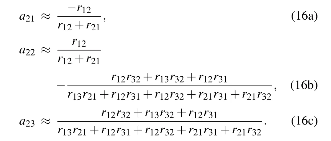
When t=0,with the initial conditions p1(0)=1,p2(0)=p3(0)=0 and the low transition rates approximation,we can get the expressions of the coefficients of a21,a22and a23as follows:

Then the auto-correlation function g2(t)can be written as[22]

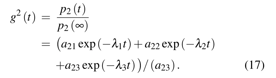
By substituting the parameters in Eq.(17),g2(t)can be written as

4.Summary