Logistic扩散过程中漂移系数的序列极大似然估计

叶 菁

(四川大学数学学院, 成都 610064)

1 Introduction

In this paper, we study a sequential maximum likelihood estimator (SMLE) of the unknown drift parameter for the following Logistic diffusion process

dXt=αXt(1-βXt)dt+σXtdWt,

X0=x0>0

(1)

where {Wt,t≥0} is a standard Wiener process on a complete filtered probability space (Ω,F,(Ft,t≥0),P) with the filtration (Ft,t≥0) satisfying the usual conditions. SupposeX(t) represents a population density at timet. The intrinsic growth rateαis the unknown parameter to be estimated on the basis of continuous observation of the processXup to a certain predetermined level of precision. The known parameterβis called the carrying capacity of the environment and usually represents the maximum population that can be supported by the resources of the environment. The known parameterσis the noise intensity which represents the effect of the noise on the dynamics ofX.

The Logistic diffusion process is useful for modeling the population systems under environmental noise, which have recently been studied by many authors[1-5]. However, if the noise is suiciently large then the population will become extinct. Therefore, it is reasonable to assume thatα>0,β>0,σ2<2α.

In this paper, we use the SMLE to estimate the unknown parameter of Logistic diffusion process. Sequential maximum likelihood estimation in discrete time has been studied in Lai and Siegmund[6], and this type of sampling plan dates back to Anscombe[7]. In continuous time processes, SMLE was first studied by Novikov[8]. He proved the SMLE of the drift parameter for a linear stochastic differential equation is unbiased, normally distributed and effective. Since then this method has been applied to estimate the drift parameter of other kinds of stochastic differential equations[9-10]. To the best of our knowledge, the probelm has not been studied for the Logistic diffusion process. In this paper, we are concerned with this topic.

The aim of this paper is to study the statistical inference for the Logistic diffusion processXgiven by Eq.(1). More precisely, we would estimate the unknown parameterαbased on a continuous observation of the state processXup to a certain predetermined level of precision by proposing to use an SMLE. We prove that the SMLE associated with the unknown parameterαis closed, unbiased, normally distributed and strongly consistent. However, it is very diicult to obtain the upper bound of the average observation time by the similar method adopted by Leeetal.[10].To overcome this diiculty, a useful computing method is proposed in this paper, based on the upper bound ofEα[1/Xt].

The rest of the paper is organized as follows. In Section 2, we introduce a sequential estimation plan for the Logistic diffusion process, and present the main theoretical results in Theorems 2.1～2.3. Section 3 is devoted to numerical studies which illustrate the eiciency of the proposed estimator.

2 Sequential maximum likelihood estimation

(2)

(3)

Moreover,we have

(i) The sequential estimator is unbiased,i.e., for eachH∈(0,∞),

whereEαdenotes the expectation operator corresponding to the probability measurePα;

(ii) For eachH>0 fixed, it holds that

whereN(0,1) denotes the standard normal distribution.In particular, we have

(iii) The sequential estimator is strongly consistent. Namely

whenH→∞.

and

(4)

we obtain the SMLE given by

(5)

To verify (i), it is enough notice that for anyT>0

and therefore, we have

which is to say that

Sinceα>0.5σ2, the Logistic diffusion processXgiven by Eq. (1) has a unique stationary distributionμ(·) on (0,∞) (see Ref.[3, Theorem 3.2]). By the ergodic theorem, we have

which implies that

The proof of (ii) follows directly from noting that

Next, the random variable

In the next theorem we get the upper and lower bounds of the average observation time under some assumptions.

Eα[τ(H)]≥

(6)

In the caseα>σ2, the following upper bound estimate holds forEα[τ(H)]

Eα[τ(H)]≤

(7)

ProofBy Itformula, we have

(8)

Settingt=τ(H) in Eq.(8), we get

[1-Xτ(H)]+(ln x0-βx0)+αH+

(9)

(10)

Hence,

Eq.(6) holds.

To deduce Eq.(7), notice that by Eq.(9) we have

(11)

Finally, sinceα>σ2, we obtain an upper bound by the Lemma 2.2 of Jiangetal.[14]

from which the desired result Eq.(7) follows using Eq.(10) and Eq.(11).

(12)

(13)

ProofThe proof is adapted from that of Theorem 7.22 in Ref.[13]. Differentiating both sides of Eq.(12) with respect toαyields that

Then, since

it follows that

namely,

(14)

Applying Cauchy-Schwarz inequality in Eq.(14), we obtain

Therefore, Eq.(13) holds.

3 Numerical illustrations

(a) setα=2,β=1,σ=1.5；

(b) setα=4,β=1,σ=1.5；

(c) setα=4,β=1,σ=1.5；

(d) setα=2,β=0.5,σ=1.5.

Tab.1 The ME of the SMLE

Fig.1 The star points are the MSE plot for the SMLE and the solid line is the corresponding theoretical MSE of the SMLE. The SMLE shows performance well

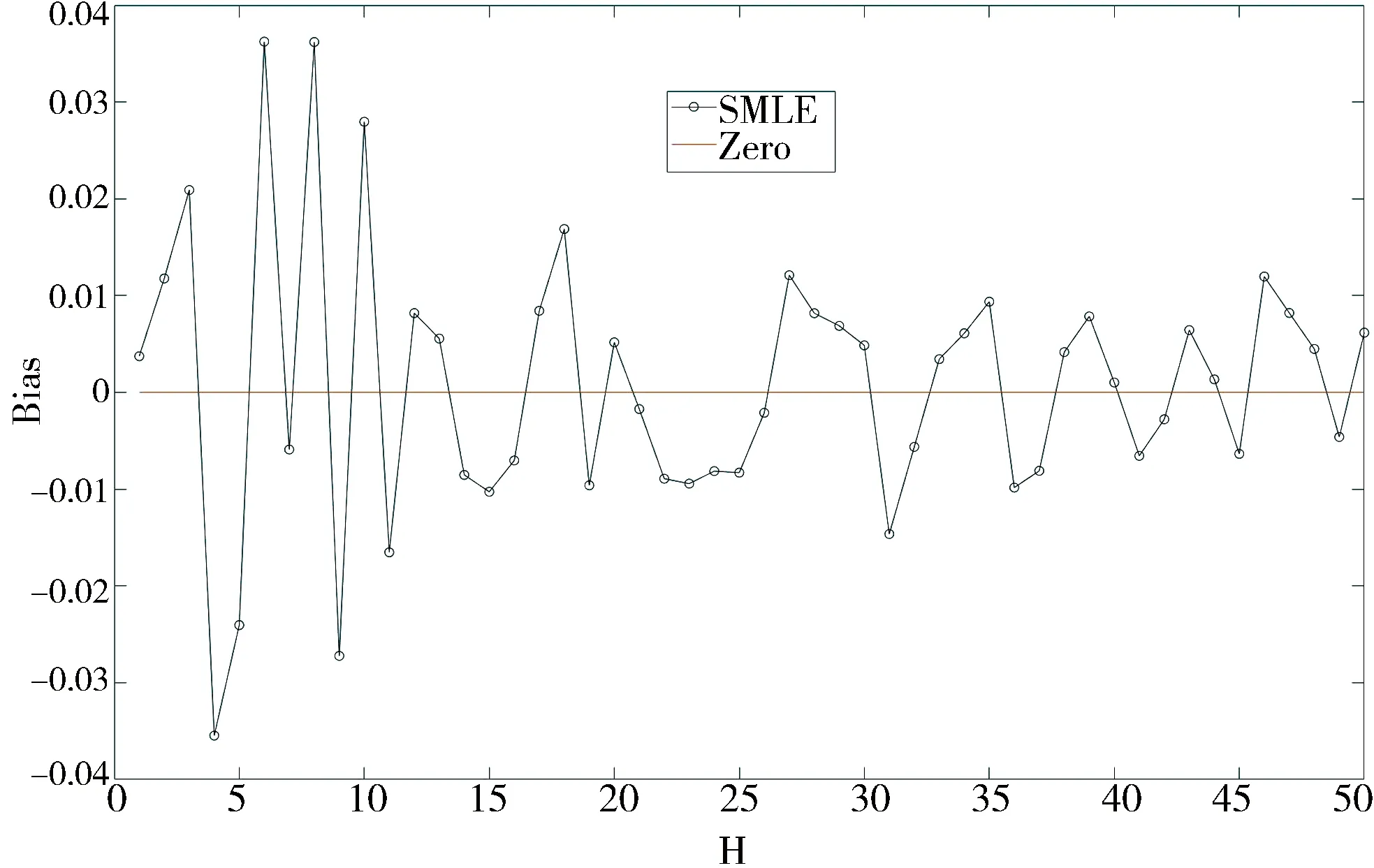
Fig. 2 Bias plot for the SMLE against H

Fig.3 Histogram of with (a) H=10 and (b) H=50， the dashed lines are the plots of the standard normal density