Facial Features of an Air Gun Array Wavelet in the Time-Frequency Domain Based on Marine Vertical Cables

ZHANG Dong LIU Huaishan 3 * XING Lei 3 * WEI Jia2 WANG Jianhua ZHOU Heng5 and GE Xinmin3 6

Facial Features of an Air Gun Array Wavelet in the Time-Frequency Domain Based on Marine Vertical Cables

ZHANG Dong1), 2), 3), LIU Huaishan1),3), *, XING Lei1), 3), *, WEI Jia2), WANG Jianhua4), ZHOU Heng5), and GE Xinmin3), 6)

1),,,,266100,2),,,266071,3),,266071,4),,100028,5),,072750,6),,266580,

Air gun arrays are often used in marine energy exploration and marine geological surveys. The study of the single bubble dynamics and multibubbles produced by air guns interacting with each other is helpful in understanding pressure signals. We used the van der Waals air gun model to simulate the wavelets of a sleeve gun of various offsets and arrival angles. Several factors were taken into account, such as heat transfer, the thermodynamically open quasi-static system, the vertical rise of the bubble, and air gun post throttling. Marine vertical cables are located on the seafloor, but hydrophones are located in seawater and are far away from the air gun array vertically. This situation conforms to the acquisition conditions of the air gun far-field wavelet and thus avoids the problems of ship noise, ocean surges, and coupling. High-quality 3D wavelet data of air gun arrays were collected during a vertical cable test in the South China Sea in 2017. We proposed an evaluation method of multidimensional facial features, including zero- peak amplitude, peak-peak amplitude, bubble period, primary-to-bubble ratio, frequency spectrum, instantaneous amplitude, instantaneous phase, and instantaneous frequency, to characterize the 3D air gun wave field. The match between the facial features in the field and simulated data provides confidence for the use of the van der Waals air gun model to predict air gun wavelet and facial features to evaluate air gun array.

air gun; van der Waals; marine vertical cable; facial features; multidimensional

1 Introduction

Air guns are the most commonly used seismic source in geophysical exploration due to their low cost and stable repeatability. With the use of an air gun, high-pressure air is released into water rapidly after firing, which produces a short duration, nearly spherical, high-energy, bottom- oriented, broadband pulse signal (Caldwell and Dragoset, 2000; Zhang., 2017; Wang., 2018). The study of air gun bubble theory is the basis for constructing an accurate air gun model, and the rational evaluation of air gun arrays is an important link in marine exploration.

Rayleigh (1917) studied the oscillation of spherical bubbles in incompressible fluid and found that collapse time was a function of hydrostatic pressure, initial bubble radius, and fluid density. This finding promoted researchers’ un- derstanding of bubble oscillation and thus prompted researchers to expand the theory (Herring, 1941; Keller and Kolodner, 1956). Herring (1941) approximated the pressure wave of the bubble as a sound wave, taking into account the energy loss caused by the radiation of the pressure wave, and derived the nonlinear wave equation and the bubble oscillation equation. Kirkwood and Bethe (1942) studied the shock waves produced by underwater explosions, considered the compressible effects of the fluid, and assumed that the velocity of the pressure waves in the fluid is the sum of the velocity of acoustic waves in the fluid and the particle velocity; this assumption is often referred to as the Kirkwood-Bethe hypothesis. Gilmore (1952) deduced the expressions of the pressure wavefield generated by bubbles in viscous compressible fluids on the basis of this hypothesis. Keller and Kolodner (1956) analyzed bubble oscillation in compressible liquids and proposed the free bubble oscillation theory to describe the motion of bubbles in seawater. Ziolkowski (1970) proposed a single air gun model on the basis of the equation of motion (Gilmore, 1952), in which bubbles oscillate in an inviscid, compressible, infinite liquid, and bubble heat transfer and jet rupture are the main factors leading to energy loss. Schulze-Gattermann (1972) established an ideal air gun source model on the basis of free bubble oscillation and emphasized the influence of the gun body on the bubble period. Ziolkowski (1982) proposed that the evaporation and condensation of bubble walls would cause heat transfer. Dragoset (1984) considered the effects of shuttle motion and the actual port size on the wavelet. Laws(1990) found that mass transmission was caused by evaporation and condensation, throttling effects, and turbulence. Landrø and Sollie (1992) added an attenuation term to the bubble oscillation equation, considered the heat transfer between the bubble and the surrounding water, and approximated the process to an open thermodynamic system. Heat transfer between the air gun and the bubble was conducted through a shuttle valve. Landrø and Sollie (1992) simplified the process of gas transfer from the air gun to the bubble and proposed a linear degassing process hypothesis. Langhammer and Landrø (1993) studied the in- fluence of the viscosity of the surrounding fluid on the air gun wavelet, and they concluded that the viscosity was not the main reason for the pressure wavelet attenuation. Li. (2010) comprehensively considered various phy- sical factors in the process of bubble oscillation, including heat transfer between the bubble and surrounding water, vertical motion of the bubble, fluid viscosity, air release time, and the effect of the air gun body. Graaf. (2014) compared the Rayleigh-Plesset and Gilmore equations, and they concluded that the most likely main reason for additional damping of air gun bubbles was the heat transfer between water and air. Moreover, they concluded that the throttling effect during air release has a significant impact on the maximum radius of bubbles and the initial pulse energy.Wang. (2015) considered that the van der Waals nonideal gas state equation could better reflect the real behavior of gas than the ideal gas state equation can.Smith and Wang (2018) considered the compressibility of fluid, surface tension, and nonlinear bubble oscillation and conducted theoretical research on bubble dynamics based on the Keller-Miksis equation (Keller and Miksis, 1980).

Modeling air gun signals is essential for assessing whe- ther the performance of an air gun array can meet the requirements of geophysical exploration. The effectiveness of various array designs can be ascertained by examining 3D radiation patterns. Musser. (1984) measured and modeled 3D far-field source radiation patterns to study theeffects of the array geometry and air gun depth. The navigation direction of the ship carrying the seismic source affects the relative position of the air gun array, thereby affecting the 3D propagation characteristics of acoustic energy relative to the azimuth of the vessel (Krail, 2010). Furthermore, for broadband signals, the acoustic transmission loss is often modeled in 1/3-octave bands. The advantage of this process is that the frequency-dependent propagation characteristics of a particular environment canbe resolved while the overall sound pressure level is computed efficiently for any receiver position (Macgillivray and Chapman, 2005).

Some air gun models, such as the air gun array source model (AASM) (MacGillivray, 2018), the Centre for Marine Science and Technology air gun array model (Cagam) (Duncan and Gavrilov, 2019), and the air gun source model (Agora) (Sertlek and Blacquière, 2019), use a variation of spherical bubble theory to solve the motion equation of air gun bubbles, follow the general dynamic theory proposed by Ziolkowski (1970), and predict the radiation source waveform. This situation shows that the spherical bubble theory is well developed and that its prediction has been widely verified by field data (Prosperetti and Lezzi, 1986). The air gun model in this paper is based on the theory of spherical bubbles, ignoring the influence of bubble deformation on bubble dynamics (Han, 2015; Zhang, 2015; Zhang, 2017) and considering the heat transfer across the bubble wall, bubble rise, throttling effect, van der Waals nonideal gas equations, and interactions between oscillating bubbles (Herring, 1941; Ziolkowski, 1982; Strandenes and Vaage, 1992; Lang- hammer and Landrø, 1993; Li, 2010; Wang., 2015; Zhang., 2016). Different types of air guns require different tuning parameters. The sleeve gun is taken as the simulation object to simulate the 3D wavefield recorded by a marine vertical cable, and a series of evaluation parameter profiles of interest is generated to evaluate the performance of the air gun array. The 3D wavefield characteristics of the model are verified by the collected vertical cable data.

2 Working Principle of the Sleeve Air Gun

In 1983, the Western Geophysics Company introduced sleeve guns that have the advantages of simple structure, good durability, and good repeatability. The 360˚ annular opening structure of the sleeve gun avoids the instability caused by the release of porous gas, the generated bubbles are closer to the sphere, and the wavelet bandwidth is significantly improved (Allen, 1987; Fontana and Haugland, 1991).

The working principle of the sleeve air gun is shown in Fig.1. In the charged state, due to the effect of high-pressure air in the return chamber, the shuttle valve is pushed to slide toward the main air chamber, the exhaust port of the main air chamber is closed, and the high-pressure gas in the high-pressure intake pipe will inflate to the main air chamber through the main air path. When the pressure in the main chamber reaches the preset rated pressure, the shuttle valve achieves dynamic balance, and inflation is completed while waiting for the firing command (Fig.1a). In the discharged state, when the solenoid valve receives the firing pulse from the gun controller, the solenoid valve is opened to let high-pressure air into the firing chamber, which breaks the mechanical dynamic balance of the shuttle valve and cause it to slide toward the back cavity, the main air chamber outlet is thus opened, releasing high-pres- sure air in the main air chamber and the return chamber into the water quickly, producing the main pulse (Fig.1b).

Fig.1 Inner structure of the sleeve gun. (a),charged state; (b),fired state.

3 Sources of Data

3.1 Marine Vertical Cable Observation System

The far-field wavelet refers to the wavelet received at a certain distance from the air gun array, that is, the distance when the propagation time of all single guns from the array is a few milliseconds apart or when the ratio of the sea surface reflection amplitude to the direct wave amplitude is greater than 95% (Dragoset and Cumro, 1987). Generally, far-field wavelet measurements must be carried out 200–300m or more below or near the air gun array. Most marine seismic exploration projects are conducted on the continental shelf with a water depth of 25–200m.Therefore, in conventional exploration projects, directly measuring the far-field characteristics is usually impossible even if the water depth is more than 200m. The problem to be solved in this case is how to measure the far- field characteristics of air gun arrays.

Obviously, observing omnidirectional, multivertical airgun far-field wavelets by using traditional ocean exploration methods is not practical; such methods require the re- ceiving cable to be sunk in deep seawater (Fig.2a).The ver- tical cable can avoid the influence of surge and ship noise, improve the signal-to-noise ratio and resolution of marine seismic data acquisition, and receive the air gun wavelet signal with a high vertical angle from any azimuth, which meets the condition of recording air gun far-field wavelet (Asakawa., 2011, 2015; Guo., 2018).A circular trajectory is usually considered to be the best implementation plan (Fig.2b), but in the actual implementation sche- me, it usually navigates along multiple survey lines to obtain a real 3D air gun wavelet field, which can be used for the analysis of the spatial distribution characteristics.

The vertical cable system is mainly composed of a moo- ring buoy, pressure-resistant float, acoustic releaser, cement weight, 3 ultrashort baselines, 12 hydrophones, and 6 digital packages. Digital packages are connected by a signal synchronization line. Each digital package is connected to 2 hydrophones with an interval of 25m, a vertical cable length of 300m, and a maximum working water depth of more than 2000m (Fig.3). The depth of the vertical cable can be adjusted in real-time during the sea test, and the hydrophone interval of the vertical cable is not fixed and can be adjusted according to the needs of different detection targets. Vertical cables are truly digitized, with a variety of options for time sampling rates of 4, 2, 1, 0.5, 0.25, and 0.125ms and a frequency bandwidth of 10Hz–8kHz for the hydrophone signal.

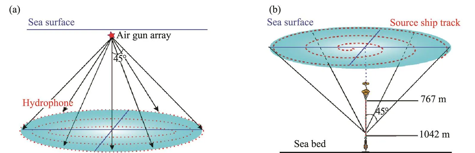
Fig.2 Different observation methods of far-field wavelets. (a),traditional observation mode (scheme not feasible); (b),vertical cable observation mode (scheme feasible).

3.2 Marine Vertical Cable Experiments in the South China Sea

In April 2017, the team conducted an ocean vertical cable acquisition test at a depth of 1200m in the South China Sea. The source of the air gun is composed of four air guns with a total capacity of 540inch3(8.85L) and arranged into two subarrays with a spacing of 1.6m(Fig.4). The air gun has a firing pressure of 138MPa, and the array has a drag depth of 5m. The hydrophone is suspended in seawater at a depth of 767–1042m by anchoring the ocean vertical cable to the seafloor and relying on buoys to maintain a state nearly perpendicular to the seafloor. The air gun source is shot along the line with a spacing of 25m, and the signals above and around the vertical cable are collected according to the predetermined mode with a sampling interval of 0.25ms. Fig.5 shows a schematic of vertical cable stereoscopic observation. The source ship travels along the line, the arrow represents the ship’s direction of navigation, the adjacent line of the navigation trajectory interval is 100m, the line area is formed by 33 lines of the 3D vertical cable data range, and the vertical cable is in the central position.

Fig.3 Vertical cable recording system.

Fig.4 Air gun array configuration.

4 Wavelet Simulation Process of Air Guns Based on the van der Waals Equation

4.1 van der Waals Equation

For different types of air guns, the traditional wavelet model of air guns assumes that the high-pressure gas in the air gun is the ideal gas, which satisfies the ideal gas state equation:

wherePgis the air gun chamber pressure, Vg is the chamber volume of the air gun,mg is the mass of high-pressure air,Rg is the universal gas constant, andTg is the temperature of the air in thechamber.

The ideal gas law is relatively accurate at normal temperature and pressure, but when the gas temperature or pressure is too high, the ideal gas equation will not be applicable. In fact, the pressure inside the gun body of the air gun source is very large, which is generally above 100 MPa. The simulation of air gun source wavelets by using the ideal gas wavelet model will inevitably cause errors. Therefore, the more accurate van der Waals gas equation isintroduced into the simulation of the air gun source wavelet. The van der Waals gas equation is modified based on the ideal gas equation, which can describe the change process of gas more accurately. The van der Waals gas equation is as follows (Tsien, 1947):

where=0.1404m6Pamol−2and=3.764×10−5m3mol−1are the van der Waalscorrection constants.

4.2 Initial Conditions in the Simulation Process

The initial parameters of the van der Waals airgun mo- del include the following.

1) Environmental parameters: standard atmospheric pressureatm, reference pressure constantcon, seawater density,gravity acceleration, airgun depth, bubble hydrostatic pressure∞=atm+, seawater temperatureT, acoustic velocity in seawatersea, and sea surface reflection coefficientR.

2) Simulated wavelet parameters: time length of airgun waveletmax, time sampling interval∆.

3) Parameters in the van der Waals equation and quasi-static thermodynamic system: van der Waals correction constantsand, specific heat capacities at constant pressureC, specific heat capacities at constant volumeC, and universal gas constantR=C−C.

4) Calibration parameters of the air gun: heat transfer coefficient, air release ratio,volume-independent port throttling constant, and throttling power law exponent.

5) Parameters of air gun chamber: chamber capacity of air gun V, airgun pressureP, initial temperature of the air in the chamberT=T(1+P/con)(Laws, 1990), mass of the air in the chamberm, and initial value mcalculated by Eq. (2).

6) Parameters of bubbles: initial volume of bubbles produced by air released from air gun chamberV, with an initial valueV; initial radius of the bubbleR=(3V/4π)1/3; initial velocity of the bubble wall=0; bubble temperatureT, with an initial value equal to T; initial bubble pressurePequal to the hydrostatic pressure∞; and mass of the air in the bubble, with an initial value equal to=∞V/RT.

4.3 Simulation Process of Single Air Gun

1) Set the initial conditions.

whereis the volume-independent port throttling constant,is the throttling power law exponent,m0is the initial mass of the air, andis the air release ratio.

4) Calculate the change rate of the bubble volume:

5) Calculate the temperature change rate of bubbles by using the quasi-static open thermodynamic system equation

8) Calculate the bubbleradius,bubblevolume, radial velocity, air temperature, mass of air in the bubble, and mass of air in the chamber by using an iterative algorithm based on appropriately truncating Taylor seriesexpansions:

9) Calculate the air pressure in the bubblePand the chamber pressurePby using the van der Waals equation of state:

10) The vertical velocity of the bubble was calculated by Herring (1941):

11) Calculate the hydrostatic water pressure∞at the next moment:

12) Calculate the radiated pressure, which can be expressed as a function of the enthalpy, bubble wall velocity, and bubble radius (Gilmore, 1952):

whereis the distance from the bubble center to the receiving point.

13) Repeat steps 2 to 12 until>max.

14) Calculate the acoustic pressure, including thecon-tribution from the surface ghost, using image theory as follows:

4.4 Simulation Process of Air Gun Array

The interaction between the bubbles changes the pressure field of each bubble. In this paper, a time-related term is introduced into the expression to represent the effective hydrostatic pressure around each bubble (Ziolkow- ski., 1982). Thus, the effective hydrostatic pressure of theth bubble becomes

whereris the distance from gunto gun, andR,H, anduare the radius, enthalpy, and velocity of bubble, respectively.

4.5 Comparison

To verify the accuracy of the simulation results, air gun wavelets with different horizontal distances, azimuth angles, and take-off angles recorded at different depths are simulated and compared with the air gun wavelets recorded by the vertical cable. The positions of the vertical cable hydrophone and air gun are shown in Fig.6, and position parameters are shown in Table 1.

The air gun releases a large amount of high-pressure air into the water in a short period of time, generating a long rise time pulse and a low-frequency oscillation bubble. The low-frequency content increases with the rise time, while the slope and high-frequency content decrease,which provides better seismic penetration and significantly improvesseismic imaging. Fig.7 shows the time-frequency comparison results of the simulated air gun wavelet and the mea- sured air gun wavelet recorded by the marine high-precision vertical cable stereo observation system. The main pulse and low-frequency content of the measured wavelet matched the modeled signals. Therefore, the air gun wavelet simulation will have obvious advantages in seismic imaging, in establishing a full waveform inversion velocity model, and in other applications. The mismatch between the modeled data and the measured data is not surprising because predicting the far-field signature at high take-off angles and at higher frequencies from modeling is notoriously difficult. In fact, many uncertain factors are not considered in the simulation process, including the change in acoustic wave velocity in the seawater, the sea surface roughness, and the error of the position data of air guns and hydrophones, which will affect the accuracy of the simulation results.

Fig.6 The geometry of four different air gun array positions and three different depth hydrophones (three hydrophone depths are −842m,−892m and −992m respectively).

Table 1 Position information of air gun and hydrophones

Note: The data are horizontal distance between hydrophone and the air gun array, azimuth angle, take- off angle, respectively.

Fig.7 Comparisons between the measured (blue lines) and simulated (red lines) far-field wavelets (left panels) and their frequency spectra (right panels) from the air gun array in different positions at different receivers. (a), the depth of hydrophone 1 is 842m; (b), the depth of hydrophone 2 is 892m; (c), the depth of hydrophone 3 is 992m.

5 Facial Features of the Simulated Acous- tic Field Recorded by a Marine Vertical Cable Under Actual Conditions

The acoustic energy distribution and the directivity of an air gun array reflect its stability along different vertical angles and azimuths and are important parameters to eva- luate the data quality (Loveridge., 1984; Hatton and Haddow, 1991). The wave field of the air gun is simulated according to the actual spatial position of the air gun and the hydrophone with a depth of 817m and considering the influencing factors of the navigation direction. The subjects of this study are the following: generation of the wavelet facial features’ evaluation parameter profiles covering the near- and far-field wavelet and a set of vertical planes, including the far-field wavelets, the frequencyspectrum, and the instantaneous attribute with different horizontal azimuth angles, which allows the generation of zero-peak amplitude (the amplitude of the first positive pressure pulse produced after the release of the high-pressure air); the peak-peak amplitude (the difference between the first positive and the first negative pressure pulses); the bubble period (the time interval between the main pulse and the first bubble pulse), the primary-to-bubble ratio (the ratio of the first pressure pulse amplitude to the first bubble pulse amplitude); and the energy distribution at different frequencies in 3D space.

Fig.8a shows the air gun array simulated herein; the parameters of the array can be found in Section 3.2. The notional signatures of the three air guns with different volumes are shown in Fig.8b. An individual air bubble oscillates with a period related to volume and other parameters. The far-field wavelet shows that the zero-peak amplitude is 7.1barm, the peak-peak amplitude is 13.2barm, and the primary-to-bubble ratio is 5.2 (Fig.8c). The power spectra, which can be used to reveal the bandwidth of the wavelet, the energy distribution in different frequency ranges, the reflection from the sea surface, and the bubble oscillation characteristics, are important features in evaluating an air gun array. Power spectra analysis demonstrates that the low-frequency spectrum oscillations of the far-field wavelet fired by the square array are small and smooth, with better stability than that of a single gun (Figs.8d and 8e).

The energy distributions of the far-field wavelet in the two directions are similar, as shown in Figs.8f and 8g. With the far-field wavelet parallel to the navigation direction taken as an example, the broadband (0–500Hz) directi- vities of the source primarily yield the downward focusing effect of this geometry. Particularly at higher frequencies, the energy attenuates gradually as the vertical angle of incidence and the notch frequency increase and the frequencyband widens (Fig.8h). The waveform of the far-field wave- let and its variation are important parameters for evaluating the air gun source. The waveform is a comprehensive reflection of the amplitude, phase, and frequency of the response parameters. The variations in the waveform directly affect the parameters of the wavelet, including the number of peaks and troughs, the increases and decreases in the amplitude, the concavity and convexity, and the cha- racteristics of extreme points and inflection points. Therefore, instantaneous attributes can be employed to effectively identify the waveform and reveal additional details, which are helpful for evaluating the wavelet. The instantaneous amplitude is a statistic of pulse intensity, which can reflect the instantaneous change in the energy independent of the phase, but judging this condition on the basis of a continuous wavelet is difficult. Moreover, the instantaneous amplitude cannot reflect slight transversechanges in the wavelet with different offset distances, there- by easily causing human errors. Fig.8i demonstrates that the energy concentration distribution in the range of the vertical azimuth is 0˚–30˚. The waveform depends on the phase, and the phase shape will become distorted due to the effects of ghost wave interference and bubble oscillations. Meanwhile, the instantaneous phase can reflect the continuity of transverse changes in the far-field wavelet. Even though the wavelet energy is weaker, the instantaneous phase can also reveal more details and determine whether the far-field wavelet is continuous and whether the phase period change is small (Fig.8j). The instantaneous frequency represents the change in the instantaneous phase with time with a high-frequency resolution. Both the instantaneous frequency and the width of the main pulse of the wavelet are correlated with the wavelet resolution, which is independent of the peak frequency of the amplitude spectrum. With an increase in the vertical angle of incidence, the main pulse width decreases and the instantaneous frequency and the resolution of the wavelet increase (Fig.8k).

The 3D distribution of zero-peak amplitude is approximately circular, with weak directivity (Fig.8l), similar to peak-peak amplitude (Fig.8m). The range of the bubble period is near 79ms, and the overall trend decreases with an increase in the incident angle (Fig.8n). A large primary- to-bubble ratio corresponds to a high signal-to-noise ratio and thus improved wavelet and the wavelet spectrum. The distribution of the primary-to-bubble ratio is approximately radially symmetric, and the ratio value increases with the angle of incidence (Fig.8o). Figs.8p and 8q show that the energy distributions of far-field wavelets with frequencies of 30Hzand 60Hz are approximately radially symmetric. Thus, the energy distribution can effectively indicate the directional weakness of an air gun array and could meet the requirements for point sources in marine seismic pro- specting.

6 Facial Features of Measured Data

The data used in this article are composed of far-field wavelets of air gun array (Fig.9a)recorded by a hydrophone deployed at a depth of 817m. The 3D region represents the actual area of data acquisition. Thus, we extract a square area containing 33 lines, the center of which is the vertical cable (Fig.5). The hydrophone attached to the vertical cable is located in a deep-water environment, which is why the hydrophone can record a far-field wavelet signal similar to a strong impulse with a high resolution and signal-to-noise ratio.

The zero-peak amplitude is 6.9barm, and the peak-peak amplitude is 13.1barm(Fig.9b). The spectral curve of the far-field wavelet is slightly oscillatory because of the impacts of other marine uncertainties, and the notch frequency is 143Hz (Fig.9c). The source wavelet and ghost wavelet can be seen in the time domain (Figs.9d and 9e). With increases in the propagation distance and the vertical angle of incidence, the morphological variation in the far-field wavelet is very small, and the main pulse energy of the far-field wavelet attenuates slowly. In addition, the negative pulse time of the virtual reflection moves toward the main pulse time. The energy and directional characte- ristics of the measured far-field wavelets in different headings are in accordance with those of the simulated far-field wavelets (Figs.8f and 8g), as shown in Figs.9d and 9e. Fig.9f shows the frequency spectrum of the measured far-field wavelets. The power spectra of the measured far-field wave-lets match those of the simulated far-field wavelets (Fig.8h) at frequencies lower than 400Hz, whereas poor matching is observed at frequencies above 400Hz. These differences are attributed to the frequency response range of the receiving instrument, uncertain marine environmental factors,and inaccurate positions of air guns and hydrophones. The instantaneous attributes of the measured far-field wavelet (Figs.9g, 9h and 9i) coincide well with those of the simulated far-field wavelet (Figs.8i, 8j and 8k). In phase displays, the phases corresponding to each peak, trough, and zero-crossing of the wavelet are assigned the same color. Thus, any phase angle can be ascertained from the wavelet with different vertical angles of incidence. The phase period of the main pulse of the far-field wavelet matches well with the simulation results (Fig.9h). In addition, the instantaneous frequency (Fig.9i) seems to be noisier than the instantaneous amplitude (Fig.9g) because the phase changes more rapidly than the amplitude.

Fig.8 Simulated wavelet facial features at 5m with a square array of four single guns with a total capacity of 540inch3 (8.85L). (a), air gun array; (b), near-field wavelets of single guns with different capacities; (c), far-field wavelet; (d), near-field wavelet spectrum of single guns with different capacities; (e), far-field wavelet spectrum; (f), far-field wavelet with an azimuth of 149˚; (g), far-field wavelet with an azimuth of 59˚; (h), far-field wavelet spectrum with an azimuth of 149˚; (i), Instantaneous amplitude of the far-field wavelet with an azimuth of 149˚; (j), instantaneous phase of the far-field wavelet with an azimuth of 149˚; (k), Instantaneous frequency of the far-field wavelet with an azimuth of 149˚; (l), 3D distribution of the zero-peak amplitude; (m), distribution of the peak-peak amplitude in 3D space; (n), bubble period distribution of far-field waves in 3D space; (o), 3D distribution of the primary-to-bubble ratio; (p), energy distribution with the azimuth (30Hz); (q), energy distribution with the azimuth (60Hz). Arrows indicate the course of the source ship.

Fig.9 Measured wavelet facial features at 5m with a square array of four single air guns with a total capacity of 540inch3 (8.85L). (a), air gun array; (b), far-field wavelet; (c), far-field wavelet spectrum; (d), far-field wavelet with an azimuth of 149˚; (e), far-field wavelet with an azimuth of 59˚; (f), far-field wavelet spectrum with an azimuth of 149˚; (g), instantaneous amplitude of the far-field wavelet with an azimuth of 149˚; (h), instantaneous phase of the far-field wavelet with an azimuth of 149˚; (i), instantaneous frequency of the far-field wavelet with an azimuth of 149˚; (j), distribution of the zero-peak amplitude in 3D space; (k), energy distribution with the azimuth (30Hz); (l), energy distribution with the azimuth (60Hz). Arrows indicate the course of the source ship.

Extracting the bubble period and the primary-to-bubble ratio of a far-field wavelet in 3D space is difficult because of the influences of various uncertainties associated with marine environmental factors. Thus, we extract only the characteristics of the energy and frequency of the wavelet. The zero-peak amplitude of the measured far-field wavelet is displayed in Fig.9j. The position of the air gun relative to the vertical cable changes because of the influences of different navigation directions. As a result, the energy distribution of the far-field wavelet is biased toward the left (Fig.9j) in the vicinity of shot lines 1–9, 16–17, and 25–30 because the small-volume air gun is near the side of the ship, whereas the large-volume air gun is far from the side of the ship in this region. Furthermore, the energies of the measured far-field wavelet at different frequencies in 3D are approximately radially symmetric, which is similar to the energies of the simulated far-field wavelet (Figs.9k and 9l). The collected vertical cable data validate the model pre- diction of 3D air gun array characteristics.

7 Conclusions

This paper presents a simulation process of the van der Waals air gun wavelet under actual conditions and compares the van der Waals air gun wavelet with the mea- sured air gun wavelet of different azimuth angles, take-off angles, and horizontal distances in the time-frequency domain recorded by a marine high-precision vertical cable stereo observation system. The results show good consistency; the uncertainty of environmental factors, inaccurateposition of air guns and hydrophones, and model parameters will affect the accuracy of the calculation results. Thispaper proposes and establishes a quantitative, multidimensional representation method of air gun array wavelet si- mulation facial features in the time, space, and frequency domains. The facial features of the 3D air gun wave field measured on a marine vertical cable are in good agreement with those of the simulated results. Therefore, this evaluation provides a fairly accurate prediction of the physical parameters of the 3D acoustic field, thus possibly aiding in the optimization of the design of the air gun array, and we are free to design and optimize air gun arrays that meet the time-frequency domain needs of marine seismic exploration.

Acknowledgements

This work has been supported by the National Natural Science Foundation of China (Nos.91958206,91858215), the National Key Research and Development Program Pilot Project (Nos.2018YFC1405901, 2017YFC0307401), the Fundamental Research Funds for the Central Universities (No. 201964016) and the Marine Geological Survey Program of China Geological Survey (No. DD20190819). All authors of this manuscript do not have a conflict of interest to declare.

Allen, T. J., Jeffery, S. J., and Mansfield, G. C., 1987. Sleeve guns and wide tow., 18 (2): 1-3.

Asakawa, E., Murakami, F., Sekino, Y., Okamoto, T., Ishikawa, K., Tsukahara, H.,., 2012. Development of vertical cable seismic system.. Copen- hagen, P008.

Asakawa, E., Murakami, F., Tsukahara, H., Mizohata, S., and Tara, K., 2015. Vertical cable seismic surveys for SMS exploration in Izena Cauldron, Okinawa-Trough.Genova, 1-5.

Caldwell, J., and Dragoset, W., 2000. A brief overview of seismic air-gun arrays., 19 (8): 898-902.

Dragoset, W., 1984. A comprehensive method for evaluating the design of airguns and airgun arrays., 3(1): 856.

Dragoset, W. H., and Cumro, D. L., 1987. Method for determining the far-field signature of an air gun array. US4658384A, US.

Duncan, A. J., and Gavrilov, A. N., 2019. The CMST airgun arraymodel–A simple approach to modelling the underwater sound output from seismic airgun arrays., 44 (3): 589-597.

Fontana, P. M., and Haugland, T. A., 1991. Compact sleeve-gun source arrays., 56 (3): 1359.

Gilmore, F. R., 1952. The growth or collapse of a spherical bubble in a viscous compressible liquid. California Institute of Te- chnology Hydrodynamics Laboratory.Pasadena, CA, Report no. 26-4.

Graaf, K. L. D., Penesis, I., and Brandner, P. A., 2014. Modelling of seismic airgun bubble dynamics and pressure field using the gilmore equation with additional damping factors., 76 (1): 32-39.

Guo, Z. W., Liu, J. X., Liao, J. P., and Xiao, J. P., 2018. Compa- rison of detection capability by the controlled source electromagnetic method for hydrocarbon exploration., 11 (7): 1839.

Han, R., Zhang, A., and Liu, Y., 2015. Numerical investigation on the dynamics of two bubbles., 110:325- 338.

Hatton, L., and Haddow, K., 1991. The effects of source array crossline directivity on 3D migration., 9: 427-431.

Herring, C., 1941. Theory of the pulsations of the gas bubble produced by an underwater explosion. U.S. National Defence Research Committee, Report no. 236.

Keller, J. B.,and Kolodner, I. I.,1956. Damping of underwater explosion bubble oscillations., 27 (10): 1153-1156.

Keller, J. B., and Miksis, B., 1980. Bubble oscillations of large amplitude., 68 (2): 628-633.

Kirkwood, J. G., and Bethe, H. A., 1942. The pressure wave produced by an underwater explosion. Office of Scientific Research and Development. Report no. 588.

Krail, P. M., 2010. Airguns: Theory and operation of the marine seismic source.Course notes for GEO-391: Principles of seismic data acquisition. University of Texas at Austin. Austin, 1- 44.

Landrø, M., and Sollie, R.,1992. Source signature determinationby inversion., 57 (11): 1410.

Langhammer, J., and Landrø, M.,1993. Experimental study of viscosity effects on air-gun signatures., 58 (12): 1801-1808.

Laws, R.M., Hatton, L., and Haartsen, M., 1990. Computer mo- delling of clustered airguns.,8(9): 331-338.

Li, G.F., Cao, M.Q., Chen, H.L., and Ni, C.Z., 2010. Modeling air gun signatures in marine seismic exploration considering multiple physical factors.,7(2): 158-165.

Loveridge, M., Parkes, G., Hatton, L., and Worthington, M., 1984. Effects of marine source array directivity on seismic dataand source signature deconvolution., 2 (7): 16-22.

Macgillivray, A. O., 2018. An airgun array source model accounting for high-frequency sound emissions during firing–Solutions to the IAMW source test cases., 44 (3): 582-588.

Macgillivray, A. O., and Chapman, N. R., 2005. Results from an acoustic modelling study of seismic airgun survey noise in Queen Charlotte Basin. University of Victoria. Victoria, Report, 1-42.

Musser, J. A., Dunbar, J. A., and Fricke, J. R., 1984. Measured and modeled 3-D far-field radiation patterns for three large marine air gun arrays.. Atlanta, 280-282.

Prosperetti, A., and Lezzi, A., 1986. Bubble dynamics in a compressible liquid. Part 1. First-order theory., 168 (1): 457-478.

Rayleigh, L., 1917. On the pressure developed in a liquid during the collapse of a spherical cavity., 34 (200): 94-98.

Schulze-Gattermann, R., 1972. Physical aspects of the airpulser as a seismic energy source.,20 (1): 155-192.

Sertlek, H. Q., and Blacquiere, G., 2019. Effects of the rough sea surface on the signature of a single air gun., 44 (3): 1-7.

Smith, W. R., and Wang, Q. X., 2018. Radiative decay of the nonlinear oscillations of an adiabatic spherical bubbleat small mach number., 837: 1-18.

Strandenes, S., and Vaage, S., 1992. Signatures from clustered airguns., 10 (1258): 305-312.

Tsien, H. S., 1947. One-dimensional flows of a gas characterizedby van der Waals equation of state., 25: 301-324.

Wang, L. M., Hu, Y.,Wang, Y., Liu, B. H., and Xu, J., 2015.Source wavelet simulation of GI gun., 30: 2793-2796 (in Chinese with English abstract).

Wang, S. P., Zhang, A. M., Liu, Y. L., Zhang, S., and Cui, P., 2018. Bubble dynamics and its applications., 30 (6): 5-21.

Zhang, A. M., Cui, P., Cui, J., and Wang, Q. X., 2015. Experimental study on bubble dynamics subject to buoyancy., 776: 137-160.

Zhang, S., Wang, S. P., Zhang, A. M., and Li, Y. Q., 2017. Numerical study on attenuation of bubble pulse through tuning the air-gun array with the particle swarm optimization method., 66: 13-22.

Zhang, Y. N., Min, Q., Zhang, Y. N., and Du, X. Z., 2016. Effects of liquid compressibility on bubble-bubble interactions between oscillating bubbles., 28 (5): 832-839.

Ziolkowski, A., 1970. A method for calculating the output pressure waveform froman airgun.,21(2): 137-161.

Ziolkowski, A., 1982. An air gun model which includes heat trans- fer and bubble interactions.. Dallas, No. 520.

Ziolkowski, A. M., 1998. Measurement of air-gun bubble oscillations., 63 (6): 2009-2024.

Ziolkowski, A. M., Parkes, G. E., Hatton, L., and Haugland, T., 1982. The signature of an airgun array: Computation from near- field measurements including interaction., 47 (10): 1413-1421.

March 8, 2020;

September 10, 2020;

July 7, 2021

© Ocean University of China, Science Press and Springer-Verlag GmbH Germany 2021

E-mail: lhs@ouc.edu.cn

E-mail: xingleiouc@ouc.edu.cn

(Edited by Chen Wenwen)