
Bifurcation and dynamics in double-delayed Chua circuits with periodic perturbation
2022-02-24 09:38WenjieYang杨文杰
Chinese Physics B 2022年2期
Wenjie Yang(杨文杰)
School of Science,Xuchang University,Xuchang 461000,China
Rank-1 attractors play a vital role in biological systems and the circuit systems.In this paper,we consider a periodically kicked Chua model with two delays in a circuit system.We first analyze the local stability of the equilibria of the Chua system and obtain the existence conditions of supercritical Hopf bifurcations.Then,we derive some explicit formulas about Hopf bifurcation, which could help us find the form of Hopf bifurcation and the stability of bifurcating period solutions through the Hassards method.Also,we show that rank-1 chaos occurs when the Chua model with two delays undergoes a supercritical Hopf bifurcation and encounters a periodic kick,which shows the effect of two delays on the circuit system.Finally,we illustrate the theoretical analysis by simulations and try to explain the mechanism of delay in our system.
Keywords: rank one chaos,periodically kicked Chua model,time delay
1.Introduction
Research of chaos is a challenge in theory of nonlinear dynamical systems, especially, analyses of the global bifurcations and chaotic dynamics[1]and multi-pulse chaotic dynamics.[2]Moreover, more complex chaos attractors, such as hidden attractors, rank-1 attractors have been studied recently.For example, a rapidly growing number of studies have been published, in which hidden chaotic attractors are shown in some systems, including a single equilibrium,[3,4]stable equilibria,[5,6]as well as other systems.[7,8]Wang and Young[9]illustrated the existence of rank-1 attractors when only one direction of instability and certain external force exist,and they obtained the dual property of occurring naturally of a class of strange attractors.[10]Then Chen and Han found that a periodically kicked planar system with heteroclinic cycle having rank-1 strange attractors.[11]Also,Yanget al.proposed the rank-1 chaotic theory to solve the chaotic behavior of delayed systems,and they obtained some conditions for rank-1 chaos in a periodically kicked system.[12]
The Chua model is a well-known model to investigate the bifurcation and chaos, which has attracted more attention in recent years.[13]Tsafack and Kengne[15]pointed out that the Chua model is more flexible to show the rich dynamics behaviors.Meanwhile, Ozkaynak[16]developed a fractional-order chaotic Chua model and proved that it is crucial for the practical application of fractional-order chaotic systems.Yuet al.[17]considered some phenomena observed in a Chua system with multiple delays.
Mathematical modeling is a vital tool to study different systems and is often used to explain some novel phenomena.[18–21]Meanwhile, the concept of rank-1 attractors is used to illustrate some mechanisms and plays a vital role in biological systems and circuit systems.However, the Chua model with two delays has been seldom investigated in theory.To show the effect of two delays and a periodic kick on the Chua model, we consider a periodically kicked Chua model with two delays in a circuit system.We first analyze the local stability of the equilibria of the Chua system and obtain the existence conditions of supercritical Hopf bifurcations.Then,we derive some explicit formulas about Hopf bifurcation,which could help us find the form of Hopf bifurcation and the stability of bifurcating period solutions through the Hassards method.Also,we show that rank-1 chaos occurs when the Chua model with two delays undergoes a supercritical Hopf bifurcation and encounters a periodic kick, which shows the effect of two delays on the circuit system.Finally,we illustrate the theoretical analysis by simulations and try to explain the mechanism of delay in our system.
2.Analysis of Hopf bifurcation and rank-1 chaos in Chua model with two delays
In Ref.[20], Wang considered rank-1 chaos of the Chua model as follows:
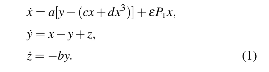
To investigate the rank-1 attractor in the Chua system with both delays and periodically kick, we add time delays τ1,τ2to Eq.(1),and obtain the following form:

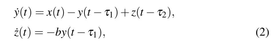
wherea,b,c,d,τ1,τ2∈R,and τ1,τ2≥0 are time delays foryandz,respectively.The undisturbed system is

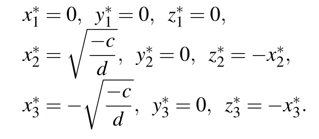
In this section, we consider system (3).It always has equilibrium,i=1,2,3,where
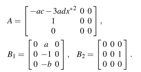
LetE∗=(x∗,y∗,z∗) denote the arbitrary equilibrium,=x(t)−x∗,=y(t)−y∗,=z(t)−z∗, still written,asx(t),y(t),z(t), respectively, then the linearized system atE∗is

whereu(t)=[x(t),y(t),z(t)]T,and
Then we think about the following three kinds of circumstances.
I.E∗=.
The characteristic equation of(4)is
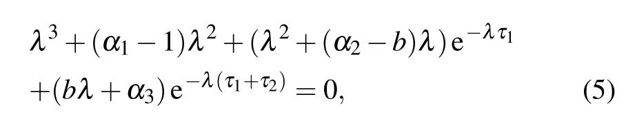
where α1=ac+1,α2=ac−a+b,α3=abc.In order to study the distribution of roots of the transcendental Eq.(5),we need to use the Corollary 2.4 of Ruan and Wei.[24]As Eq.(4) has two time delays τ1and τ2,we consider the following six cases.
Case 1:τ1=τ2=0,Eq.(5)becomes

The Routh–Hurwitz criterion implies if
(H1) α1>0,α3>0,and α1(α2−b)+b>0.
Then all roots of Eq.(5)have negative real parts.Namely,the equilibrium pointis locally asymptotically stable when the condition(H1)is satisfied.
Case 2:τ1>0,τ2=0,Eq.(5)becomes

Suppose that iω1(ω1>0) is a root of Eq.(7) in the imaginary axis.Substituting it to Eq.(7)and separating the real and imaginary parts,we have

which is equivalent to

SinceG(0)=<0,G(+∞)=+∞,we can obtain that Eq.(10)has at least one positive root sincee13<0.

According to the lemma in Ref.[23], we can investigate the distribution of the roots of Eq.(7).Sincee13<0,for the polynomial Eq.(7), we can obtain that all roots with positive real parts of Eq.(7)have the same sum to those of the polynomial Eq.(6)for τ1∈[0,τ10).
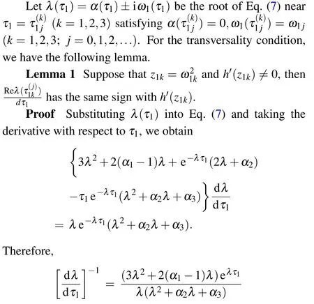
According to Eqs.(10)–(12),we have

According to the above derivation,we can obtain the following theorems.
Theorem 1Suppose that(H1)holds,
(i) when τ1∈[0,τ10), thenof system (3) is locally asymptotically stable,
(ii)when τ1>τ10,of system(3)is unstable,
(iii)when τ1=τ10,the system(3)exhibits Hopf bifurcation.
Case 3τ2>0,τ1=0.
The calculation is similar to case 2,so we have
Theorem 2Suppose that(H1)holds,
(i) when τ2∈[0,τ20), thenof system (3) is locally asymptotically stable,
(ii)when τ2>τ20,of system(3)is unstable,
(iii) when τ2=τ20, the system (3) exhibits Hopf bifurcation, where τ20is the minimum critical value of τ2for the occurrence of Hopf bifurcation when τ1=0.
Case 4τ1=τ2/=0.
Theorem 3Suppose that(H1)holds,
(i)when τ1∈[0,τ30),of system(3)is locally asymptotically stable,
(ii)when τ1>τ30,of system(3)is unstable,
(iii)when τ1=τ30,the system(3)exhibits Hopf bifurcation.
Case 5τ1>0,τ2∈[0,τ20)and τ1/=τ2.
We consider Eq.(5)with τ2∈[0,τ20),and τ1is regarded as the parameter.Let iω5(ω5>0)be the root of Eq.(5),then we can obtain

From Eq.(13),we can reach

Now we make the following assumption and get the main conclusions.
(H2): Eq.(14)has at least finite positive root.
Suppose that(H2)holds, we denote the positive roots of Eq.(14)as ω5k(k=1,2,3,4,5,6).For every ω5k, the corresponding critical value of(j=1,2,3)is

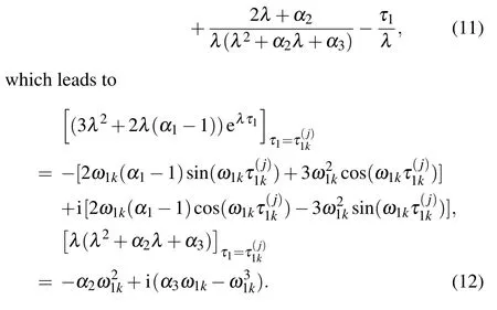
Then we differentiate two sides of Eq.(5)with respect to τ1to verify the transversality condition.Taking the derivative of λ of τ1in Eq.(5)and substituting λ =iω50,we have

which leads to

where
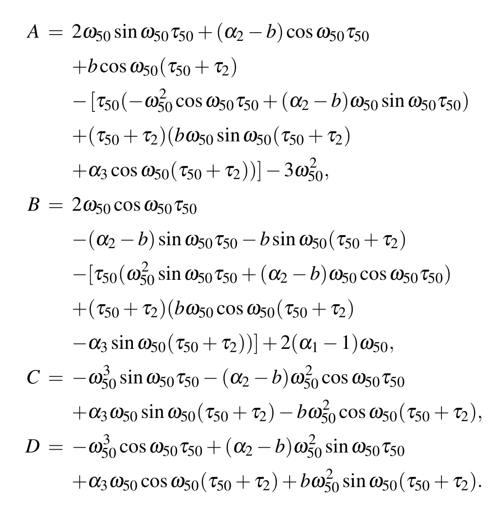
Therefore,if the following condition holds
(H3)AC+BD/=0,
Theorem 4For system (3), τ1> 0, τ2∈[0,τ20) and τ1/=τ2.Suppose that the conditions(H2)and(H3)hold,then
(i)when τ1∈[0,τ50),of system(3)is locally asymptotically stable,
(ii)when τ1>τ50,of system(3)is unstable,
(iii)when τ1=τ50,the system(3)exhibits Hopf bifurcation.
Case 6τ2>0,τ1∈[0,τ10)and τ1/=τ2.
We consider Eq.(5)with τ1∈[0,τ10),and take τ2as the parameter.The calculation is similar to case 5,so we can get the following results.
Theorem 5For system (3), τ2> 0, τ1∈[0,τ10) and τ2/=τ1.
(i)when τ2∈[0,τ60),of system(3)is locally asymptotically stable,
(ii)when τ2>τ60,of system(3)is unstable,
(iii) when τ2=τ60, the system (3) exhibits Hopf bifurcation, where τ60is the minimum critical value of τ2for the occurrence of Hopf bifurcation when τ1∈[0,τ10).
II.E∗=,or.
WhenE∗=, or, the coefficients of Eq.(5) are α1=1 −2ac, α2=−2ac−a, β1=−2ac.Under the condition (H1), Eq.(5) has at least one positive real root, soandare unstable equilibria.
3.Hopf bifurcation and rank-1 chaos of the delayed system
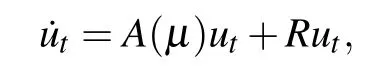
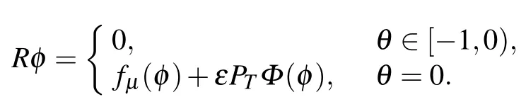
According to the above analysis, system (3) undergoes Hopf bifurcation for different τ1,τ2.Now,we apply Hassard’s method,[24]to study Hopf bifurcation of system (3) with respect to εPTx(t), τ1, τ2∈[0,τ20).Then we apply the rank-1 chaos theory to the delayed system,[12]to research the Chua model(3)with two delays and periodically kick εPT.Let τ1=τ50+µ,µ ∈R,t=sτ1,x(sτ1)=,denotex=andt=s,then system(3)with εPTx(t)(i.e.,Eq.(2))can be written as a functional differential equation(FDE)inC=C([−1,0],R3):

whereu(t)=(x(t),y(t),z(t))T∈C, andut(θ)=u(t+θ)=(x(t+θ),y(t+θ),z(t+θ))T∈CandLµ:C→R3,F:R×C→R3are given by

whereA,B1,B2are as in Eq.(4), and by the Riesz representation theorem,there is a 3×3 matrix function η(θ,µ)of bounded variation for θ ∈[−1,0],such thatLµφ as the form

In fact,we can choose

Then write Eq.(2)as
where

and

For φ ∈C([−1,0],(R3)∗), where (R3)∗is the 3-dimensional space of row vectors,andA∗is adjoint operator ofA(0):For φ ∈C([−1,0],R3),φ ∈C([−1,0],(R3)∗),and the bilinear form where η(θ)=η(θ,0),A=A(0)andA∗are adjoint operators.We have±iω50τ50that are eigenvalues ofA(0)andA∗.

Assume thatq(θ)is the eigenvector ofA(0)corresponding to iω50τ50, thenA(0)q(θ)=iω50τ50q(θ).According to the definition ofA(0),we can reach
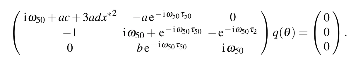
Thus,we haveq(θ)=,where
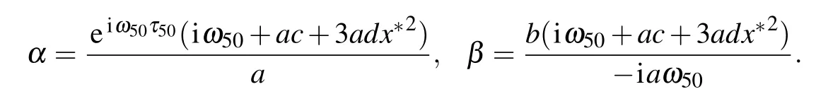
Similarly, we haveq∗(s)=that is the eigenvector to the eigenvalue −iω50τ50ofA∗, which is the adjoint operator ofA(0),where

Therefore,we have

where
such that
Then we have the coordinates to describe the center manifoldC0at τ =τ50.
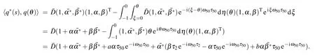
Notice thatut(θ)=(xt(θ),yt(θ),zt(θ))T=zq(θ)++W(t,θ),then we can obtain

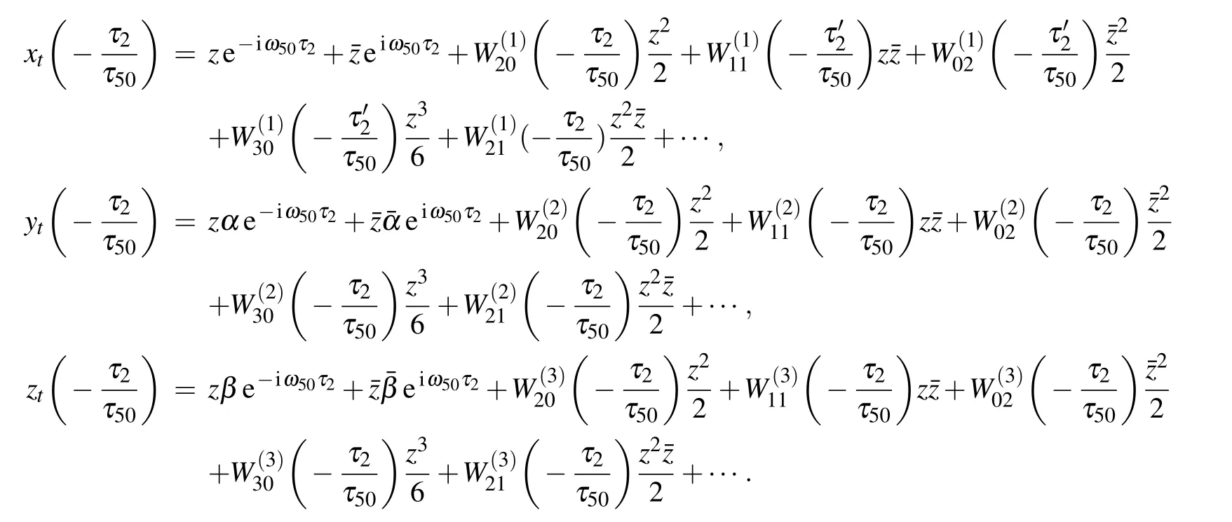
Thus,from Eq.(15)we have

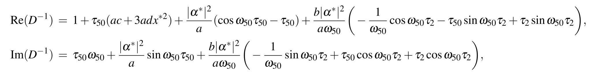
We can obtain

and

which determine the stability and bifurcation direction of periodic solutions at the critical value τ50, i.e., µ2determines the directions of a Hopf bifurcation: if Re{λ′(τ50)} > 0,µ2> 0 (resp.µ2< 0), then the Hopf bifurcation is supercritical (resp.subcritical) and the periodic solution exist for τ >τ50(τ <τ50).Here,β2determines the stability of the bifurcation periodic solutions: the bifurcating periodic solutions are stable (unstable) if β2<0 (β2>0).We can also obtain Re(k1(0))and Im(k1(0))as follows:


4.Numerical simulations
In this section, we consider the following particular example of system(2):
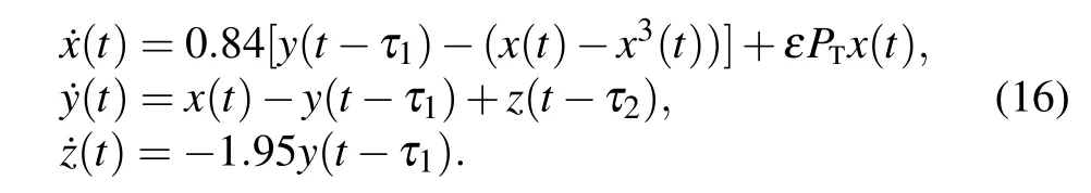
It is easy to see that(H1)holds,for τ1>0,τ2=0,we have ω10≈1.3128,τ10≈0.485.By Theorem 1,we can obtain thatE∗is asymptotically stable when τ1∈[0,τ10),when τ1passes through τ10,E∗will lose its stability,and Hopf bifurcation occurs.We can also obtaink1(0)≈−0.0457+2.3334i,µ2≈0.0431,β2≈−0.0914, so the bifurcation is supercritical and the stable periodic solution emerges fromE∗,see Figs.1 and 2.
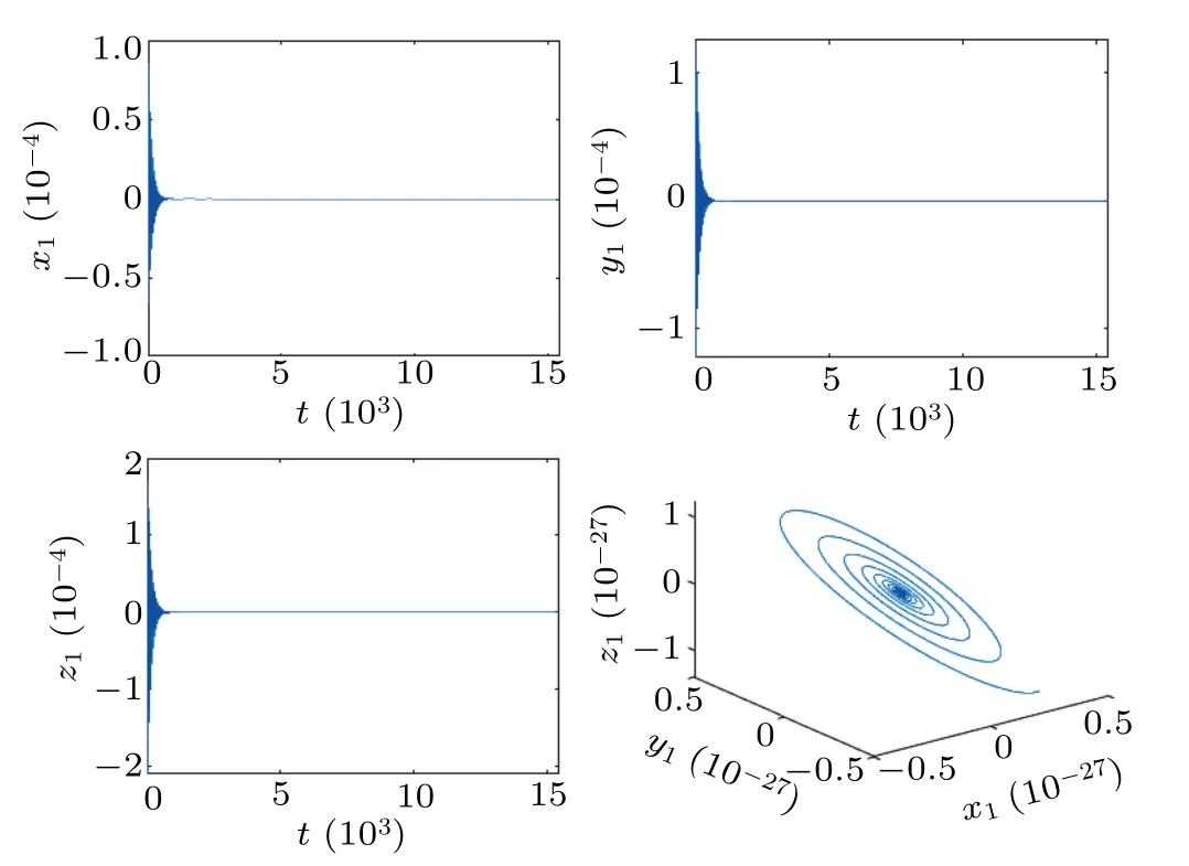
Fig.1.The trajectories and phase graphs of system (16) with ε =0,τ1 =0.4, τ2 =0. E∗becomes unstable, and a stable periodic solution bifurcates from the equilibrium E∗.
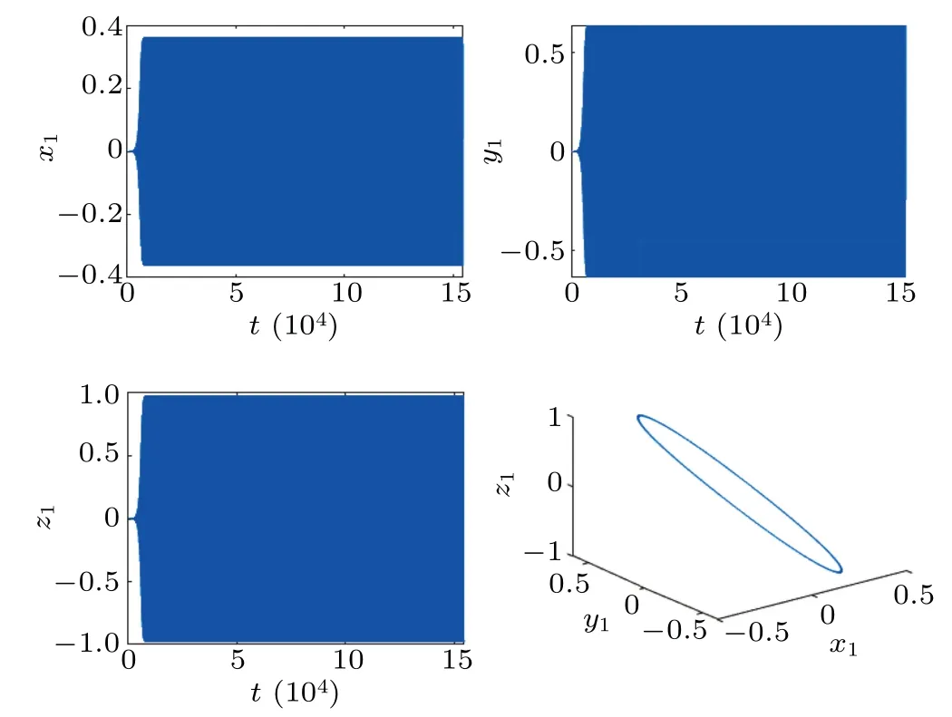
Fig.2.The trajectories and phase graphs of system (16) with ε =0,τ1=0.485,τ2=0. E∗become unstable,and a stable periodic solution bifurcates from the equilibrium E∗.

Fig.3.The trajectories and phase graphs of system (16) with ε =0,τ1 =0, τ2 =0.3. E∗becomes unstable, and a stable periodic solution bifurcates from the equilibrium E∗.

Fig.4.The trajectories and phase graphs of system (16) with ε =0,τ1=0,τ2=0.36. E∗becomes unstable,and a stable periodic solution bifurcates from the equilibrium E∗.
Similarly,for τ1=0,τ2>0,we have ω20≈1.1271,τ20≈0.3619,from Theorem 2,we can realize thatE∗is asymptotically stable when τ2∈[0,τ20).When τ2passes through τ20,E∗will lose its stability and Hopf bifurcation emerges,see Figs.3 and 4.For τ1=τ2≜τ3/=0,we can obtain ω30≈1.6186 and τ30≈1.8446.
For τ1>0,τ2=0.33 ∈[0,τ20), we have obtain ω50≈1.1554,τ50≈0.02.By Theorem 4,E∗is asymptotically stable when τ1∈[0,τ50).When τ1>τ50the steady state becomes unstable and the sustained oscillations occur.The bifurcation diagram of the system (16) forxis shown in Fig.5, where the control parameter is time delay τ1.At low values of τ1,the system reaches a stable steady state.With the increase of τ1, bifurcation occurs τ1≥0.02.We choose τ1=0.02, after the computation, we havek1(0)≈−0.0249 −0.0042i,µ2≈0.0125,β2≈−0.0498,we know that the bifurcation is supercritical and the stable periodic solution emerges fromE∗,see Figs.6 and 7.
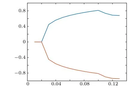
Fig.5.The bifurcation diagram of the system(16)for x.

Fig.6.The trajectories and phase graphs of system (16) with ε =0,τ1 =0.011,τ2 =0.33. E∗becomes unstable,and a stable periodic solution bifurcates from the equilibrium E∗.
For all θ such that φ′(θ)=0,φ′′(θ)/=0, we can realize that φ(θ) is a Morse function (see Fig.8), meanwhile,E(0) .=0.0249>0,|F(0)/E(0)|.=0.1686.Then we chooseT= 6897, which is quite “large” to afford us a long relaxation period between consecutive kicks of the external force.In Figs.9–11 we present a rank-1 attractor at(ε,T)=(0.73,6897),(0.73,7183),(0.93,7183) when τ1=0.02,τ2=0.33.The results of our numerical simulations well confirm the previous rank-1 theory.
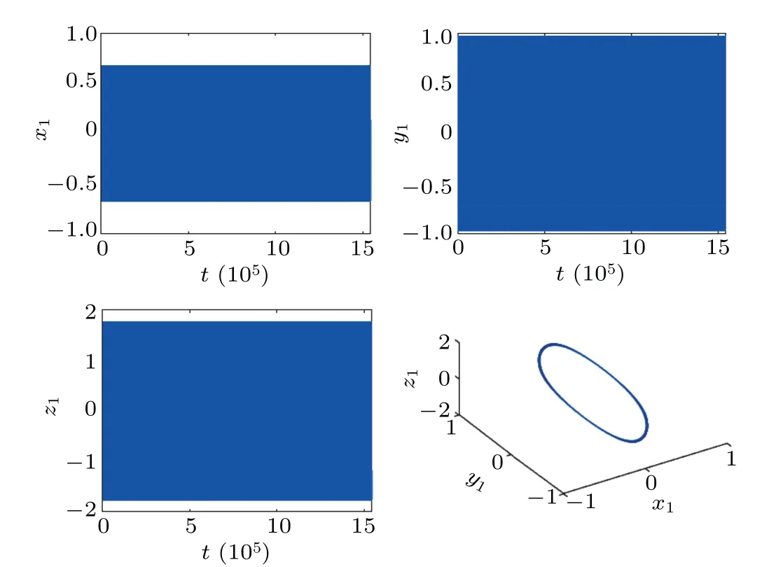
Fig.7.The trajectories and phase graphs of system (16) with ε =0,τ1=0.02,τ2=0.33. E∗becomes unstable,and a stable periodic solution bifurcates from the equilibrium E∗.

Fig.8.The graphs of φ′(θ)and φ′′(θ).

Fig.9.The trajectories and phase graphs of system(16)with T =6897,ε =0.73,τ1=0.02,τ2=0.33.A rank-1 strange attractor occurs.
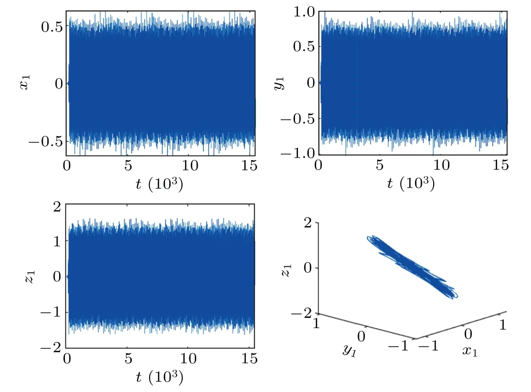
Fig.10.The trajectories and phase graphs of system (16) with T =7183,ε=0.73,τ1=0.02,τ2=0.33.A rank-1 strange attractor occurs.

Fig.11.The trajectories and phase graphs of system (16) with T =7183,ε=0.93,τ1=0.02,τ2=0.33.A rank-1 strange attractor occurs.
5.Conclusion
In summary,we have studied two-delayed Chua models.We first analyze the local stability of the system equilibria and the existence of Hopf bifurcations, and obtain the conditions that locally asymptotically stable, unstable, Hopf bifurcations occur on bases of τ1and τ2.Then we obtain some explicit formulas about Hopf bifurcation, find that µ2determines the directions of Hopf bifurcation, and β2determines the stability of the bifurcation periodic solutions.Also, we show that rank-1 chaos occurs when our Chua model with two delays undergoes a supercritical Hopf bifurcation and encounters an external periodic force,namely,suppose that φ(θ)is a Morse function and Re(k1(0))<0,rank-1 chaos occurs when>K2.Finally,we illustrate the theoretical analysis by numerical simulations.Our theoretical analysis is verified by numerical simulations,which may be a novel phenomenon to explain mechanisms of some circuits.
Acknowledgements
This work was supported by the National Natural Science Foundation of China (Grant Nos.11772291 and 12002297), Youth Talent Support Project of Henan, China(Grant No.2020HYTP012),Basic Research Project of Universities in Henan Province,China(Grant No.21zx009),Program for Science&Technology Innovation Talents in Universities of Henan Province,China(Grant No.22HASTIT018).

- Chinese Physics B的其它文章
- High sensitivity plasmonic temperature sensor based on a side-polished photonic crystal fiber
- Digital synthesis of programmable photonic integrated circuits
- Non-Rayleigh photon statistics of superbunching pseudothermal light
- Refractive index sensing of double Fano resonance excited by nano-cube array coupled with multilayer all-dielectric film
- A novel polarization converter based on the band-stop frequency selective surface
- Effects of pulse energy ratios on plasma characteristics of dual-pulse fiber-optic laser-induced breakdown spectroscopy