
A classical density functional approach to depletion interaction of Lennard-Jones binary mixtures
2022-03-23 02:21YueChenWeiChenandXiaosongChen
Yue Chen, Wei Chen and Xiaosong Chen
1 CAS Key Laboratory of Theoretical Physics, Institute of Theoretical Physics, Chinese Academy of Sciences, Beijing 100190, China
2 School of Physical Sciences, University of Chinese Academy of Sciences, Beijing 100049, China
3 State Key Laboratory of Multiphase Complex Systems, Institute of Process Engineering, Chinese Academy of Sciences, Beijing 100190, China
4 School of Systems Science, Beijing Normal University, Beijing 100875, China
Abstract In this article,we apply classical density functional theory to investigate the characteristics of depletion interaction in Lennard-Jones (LJ) binary fluid mixtures.First, to confirm the validity of our adopted density functional formalism, we calculate the radial distribution functions using a theoretical approach and compare them with results obtained by molecular dynamics simulation.Then, this approach is applied to two colloids immersed in LJ solvent systems.We investigate the variation of depletion interaction with respect to the distance of two colloids in LJ binary systems.We find that depletion interaction may be attractive or repulsive, mostly depending on the bulk density of the solvent and the temperature of the binary system.For high bulk densities, the repulsive barrier of depletion force is remarkable when the total excluded volume of colloids touches each other and reaches a maximum.The height of the repulsive barrier is related to the parameters of the LJ potential and bulk density.Moreover,the depletion force may exhibit attractive wells if the bulk density of the solvent is low.The attractive well tends to appear when the surface–surface distance of colloids is half of the size of the polymer and deepens with temperature lowering in a fixed bulk density.In contrast with the hard-sphere system, no oscillation of depletion potential around zero is observed.
Keywords: molecular simulation, density functional theory, depletion interaction, soft matter physics, colloid–polymer mixtures
1.Introduction
Classical density functional theory (CDFT) is a statistical mechanical theory for classical fluids.It originated about half a century ago [1–4], not long after quantum density functional theory (QDFT) for quantum systems was developed [5, 6].CDFT describes many-particle systems based on a variational principle in which the one-body density is the only variable,and it has found many applications in soft matter physics.The dynamical extension of CDFT, known as ‘dynamical density functional theory’(DDFT)or‘time-dependent density functional theory’,was first suggested on a phenomenological basis[7–10]and later derived from the microscopic equations of motion of the individual particles [11–15].It describes the time evolution of the one-body density.The resulting equation of motion describes the relaxation towards the equilibrium state described by CDFT and can be applied to systems that do not approach equilibrium, such as driven [16–18] or active [19–22] soft matter.In general, DDFT describes not only the equilibrium configuration, but also the dynamical behavior out of equilibrium.The early forms of DDFT were extended in a vast number of directions, making the theory applicable to systems with nonuniform temperature [23], hydrodynamic interactions[24] or superadiabatic forces [25], and to particles with inertia[26],nonspherical shapes[27]or self-propulsion[19].Although QDFT is a computationally efficient and accurate tool for exploring a wide range of issues in condensed-matter physics and chemistry [28, 29], it has limited applicability to the vast array of problems involving liquid environments, from liquid fuel-cell research to biochemistry.Therefore, methods that combined QDFT with CDFT were developed.Petrosyan et al put forward the concept of joint density functional theory(DFT)by joining an electron density functional for the electrons of a solute with a CDFT for the liquid into a single variational principle for the free energy of the combined system[30].Zhao et al proposed a reaction DFT (RxDFT) by combining the QDFT for calculation of the intrinsic reaction energy with the CDFT used to address solvation contribution and applied it to the glycine tautomerization reaction in aqueous solution [31].The satisfactory accuracy and low computational cost of RxDFT highlights its great potential for studying solvent effects on chemical reactions in solution compared with ab initio methods[32–36].Later, a dynamic reaction DFT was proposed by combining the classical dynamic DFT used to describe reactant/product diffusion with the reaction collision theory used to address chemical reactions [37].
The depletion induced interaction has attracted considerable attention due to its reasonable explanation for phenomena like phase separation, flocculation and self-assembly in colloid mixtures and colloid–polymer mixtures in colloid science [38–40], and due to its potential application to chemical engineering processes [41] and biological systems.Interestingly, the depletion interaction contains almost all the information of the phase behavior of the mixtures.When the colloids are immersed in a fluid of non-adsorbing polymers,they usually undergo depletion interaction imposed by polymers.It was first explained by Asakura and Oosawa, who modeled the colloid–polymer mixtures as hard spheres and non-interacting polymers[42].Consider the case where all of the colloids and polymers are hard spheres with diameter σband σs, respectively.The radius of the excluded volume of colloids is R=(σb+σs)/2, which is larger than that of the real volume, namely σb/2.Hence, although the volume of these hard spheres cannot overlap,their excluded volume can.The depletion of polymers produces the anisotropy of the local pressure to colloids, which causes the effective force among colloids.Subsequent studies of addictive and nonaddictive hard-sphere systems provided qualitative properties of depletion potential[43–47].The depletion force is of great importance in the basic theory of statistical mechanics since it is mainly entropy-induced if all the interactions involved between particles are the hard-sphere type [48].Also, it promoted the theory that mixtures of two species can be described equivalently by one species subjected to an effective external potential [49, 47].Hard-sphere binary mixtures are often used to model colloid–polymer mixtures and colloid mixtures [46].Instances where attractive or repulsive soft interactions are added to hard-core have also been studied[50–54].Amokrane considered a solvent–solvent Lennard-Jones (LJ) interaction and a purely hard solute–solvent potential, and showed the potential of mean force is influenced by the strength of the LJ interaction [50].Louis et al studied a model based on the hard-core Yukawa potential and observed that adding a soft repulsion to a colloid–polymer(depletant) enhanced the effective attraction between two colloids, while adding a soft attraction to a colloid-depletant interaction yielded a more remarkable repulsion between colloids [55].The methods investigating these systems [56]include computer simulation[44,45],integral equation theory[43],DFT[46,57,58]and so on.Nevertheless,the depletion interaction in the system of colloids and polymers with all interactions modeled as LJ has not been studied with CDFT.
Here,we model a colloid–polymer mixture as a binary LJ system and study the depletion effect in such a system.All the involved interactions of colloid–colloid, polymer–polymer and colloid–polymer are LJ potentials.We believe this study is beneficial in that it enables us to further understand the mechanism of depletion interaction.In our model,we refer to the ‘colloid’and the ‘polymer’as a ‘big sphere’and a‘small sphere’, respectively.The content is structured as follows:section 2 describes the DFT formalism used to investigate depletion potential and depletion force.Section 3 presents the results and discussion, in which we use DFT to calculate the radial distribution functions(RDF)of a system in which a big sphere is immersed in a sea of small spheres and we compare them with the results obtained by molecular dynamics simulation.Also, we give density profiles of small spheres around two big spheres and the depletion potential and depletion force with respect to several parameters of the colloid–polymer LJ potential, bulk densities of polymers and temperatures of systems.In section 4 we present the summary and conclusions.
2.Theory
There is no universal free energy functional applicable to all systems, hence the practical application of CDFT or DDFT requires additional approximation to construct the exact expression of the free energy functional.To make it easier for readers to understand our methods, we give a brief introduction to DFT.The basic idea of DFT [59, 60] is that the grand potential of an inhomogeneous fluid can be expressed as a functional of the average single-particle density[61–64],

whereF[ρ(r)]is the intrinsic free energy, μ is the chemical potential and V(r) is the external potential.The average single-particle density is defined by

where N is the number of particles, δ is the Dirac δ-function and the angular brackets denote an average over a grand canonical ensemble.UsuallyF[ρ(r)]is split into an ideal part and an excess part,

where the ideal intrinsic free energy can be derived as
where kBis the Boltzmann constant, and Λ is the thermal wavelengthBy minimizing the grand potential,
we can obtain the equilibrium density distribution

where β=1/(kBT), the bulk densityin which μidis the ideal chemical potential, μexis the excess chemical potential and the one-body direct correlation function

As a typical perturbation approach, the excess intrinsic free energy is split into contributions from the short-ranged repulsive potential and the long-ranged attractive potential,

The LJ potential is
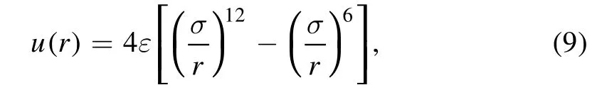
where ε and σ are the energy and length parameters,respectively.For the LJ potential among small spheres, we follow the split proposed by Barker and Henderson [65, 66].That is,the LJ potential is divided into the repulsive part with r ≤σ and the attractive part with r >σ.The repulsive part of the LJ potential is
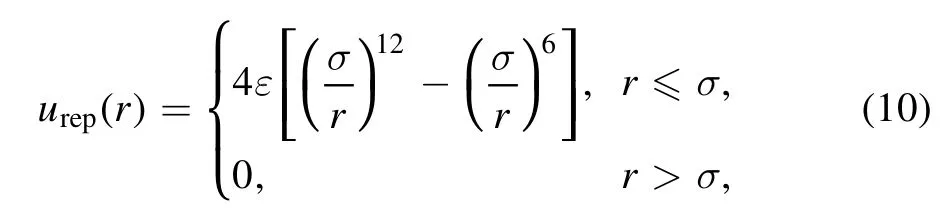
and the attractive part is

While the long-ranged attractive potential is regarded as a perturbation, the short-ranged repulsive potential is approximated as a hard-sphere potential with the effective diameter given by

which can be obtained from [67]
According to the fundamental measure theory originally proposed by Rosenfeld [68–70], the excess intrinsic free energy functional of the repulsive part can be expressed as(a system containing only a single species is considered)

where kBTΦ is the excess intrinsic free energy density,and Φ is a function of the weighted densities [68] and is given by
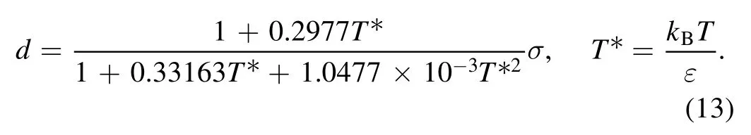
The weighted densities nα(r), α=0, 1, 2, 3 in equation (15)are given in [71, 63, 64].
From equations (7), (8), (14) and (15), the one-body direct correlation function from contribution of the repulsive potential is

With regard to the excess intrinsic free energy functional of the attractive part, we use the first-order mean-spherical approximation (FMSA) proposed by Tang and co-workers[72–76].Thus, the full one-body direct correlation function c(1)(r;[ρ(r)]) in equation (6) is obtained.
When two big colloids are immersed in a sea of small polymers, we denote the center-to-center distance of two colloids by D, which influences the grand potential of a system if it is small.However,when D →∞,the colloids are independent from each other.The depletion potential between two colloids is obtained by [46, 58]
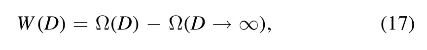
where Ω is the grand potential of the system.The depletion force is then calculated using [56]

where T is the absolute temperature.
Given an initial density distribution, c(1)(r;[ρ(r)]) can be computed using fast Fourier transform, and we can obtain a new density distribution according to equation (6).Such a numerical iteration is used to determine the equilibrium density distribution ρ(r) [77].Then, from equations (1), (3),(4), (8) and (14), we can calculate the grand potential of the system.Finally, using equations (17) and (18), the depletion potential and depletion force are obtained.
3.Results and discussion
In our calculations, there are three types of interaction:interaction among big spheres, interaction among small spheres and that between a big sphere and a small sphere.All of these interactions are described by the LJ potential but with different parameters.The energy and length parameters of the LJ potential among big spheres and among small spheres are denoted by εb, σb, εs, σs, respectively.We assume that the cross-interaction parameters follow the Lorentz and Berthelot combining rules:
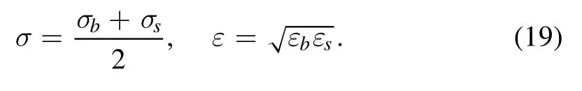
In our results, all units are reduced by the energy and length parameters of the LJ among small spheres, namely εsand σs.Therefore, we haveand(quantities with an asterisk appearing in this article denote reduced quantities).When implementing calculations of DFT, we limit particles in a cubic region with a side length of L*=50.0.
3.1.Radial distribution function
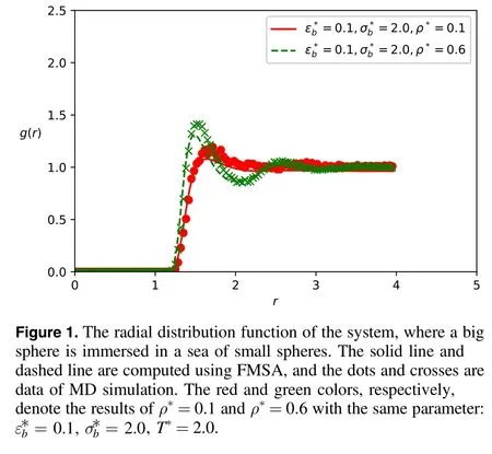
To substantiate the validity of our functional formalism in application to depletion problems in LJ systems,we calculate the radial distribution function in the case where a single big sphere is immersed in a sea of small spheres with LJ interaction among all the big and small interacting particles.We fix the single big sphere in the center of the simulation box,in which other space is occupied by small spheres and periodical boundary conditions are adopted.While=2.0 and T*=2.0, we set ρ*=0.1 and ρ*=0.6, respectively in two implementations.We compute the RDF in terms of the radial distance to the center of the big sphere and compare the results with that of molecular dynamics simulation.Using FMSA developed by Tang et al [74, 71], the RDF of the system is calculated and shown as lines in figure 1.The solid line is a result ofwith a small bulk density ρ*=0.1, and the dashed line corresponds towith a large bulk density ρ*=0.6.We can see from figure 1 that the RDF of the larger bulk density tends to have larger values when r is small and oscillates more dramatically.When r is very large, the RDF approaches the ideal gas limit, namely, approximately 1.When r ≈1.5, both RDFs have the most prominent peaks.Next, we implement molecular dynamics (MD) simulation and LAMMPS software [78, 79] is used.The results of MD are shown as dots and crosses in figure 1.We can see the overall agreement between the results of the FMSA and MD simulation,so we speculate that the functional constructed by FMSA will give a reasonable prediction of the depletion potential and the depletion force.
3.2.Structure of binary fluid
In this and the next subsection, we consider two big spheres immersed in a sea of small spheres and all the involved interactions are the LJ potential.While the LJ interaction of small spheres is treated as hard-core with an attractive tail,the interaction between big spheres and small spheres is treated as an external potential exerted on small spheres and the complete LJ potential is used.Also,in our consideration,because the time scales of motions of big and small spheres are different,i.e.the motion of big spheres is much slower than that of small spheres,we assume that the big spheres do not move at all.Therefore, the interaction between two big spheres is actually neglected.The reduced surface-to-surface distance of two big spheres isWe need to change h*to see different structures of mixtures and get a set of grand potentials.
DFT not only tells us the thermodynamical properties of a system, but it also indicates the structure of a system.To determine the density profiles of small spheres around two big spheres,we calculate= 6.0,T* = 2.0,ρ* =0.6.For each calculation, h*is respectively set to be 0.0 when two big spheres touch each other,1.0 when the excluded volumes of two big spheres touch each other and 4.0 when two big spheres are far apart.For each case,we select the density data of a middle section parallel to the YOZ plane of the entire cubic region to plot a density profile of small spheres and we show them in figures 2(a),2(b) and 2(c), respectively.The two central circular zero-density regions in figure 2 denote excluded regions of big spheres.In the region far away from two big spheres,the density of small spheres is approximately equal to the bulk density 0.6 because these small spheres are not under the influence of the external potential exerted by big spheres.What we are interested in is the nearby region of big spheres,so we select a middle section parallel to the YOZ plane from the central region of the computation box with 15.0 ≤y*≤35.0 and 18.0 ≤z*≤32.0 for h*=0.0 and 1.0,12.5 ≤y*≤37.5 and 18.0 ≤z*≤32.0 for h*=4.0.This clearer view is displayed in figure 3.We can see the regular distribution in that small spheres circle around two big spheres, forming the obvious layer structure.The structure of h*=0.0 is displayed in figure 3(a),where two big spheres contact each other.In this case,there is the largest overlap between two excluded volumes of big spheres and the total excluded volume reaches a minimum.We can see that in the region between the surface of big spheres and the innermost layer, the density of the small spheres gradually increases with the distance to the centers of the big spheres getting larger.The innermost layer formed by small spheres has a very high density ranging from 0.8 to 1.0,indicating that small spheres tend to pack around two big spheres.The second innermost layer has a density approximately equal to the bulk density 0.6.The density in the third innermost layer is higher than the bulk density but lower than that in the innermost layer.When the distance to the surfaces of big spheres can be compared with the size of big spheres,the density of the small spheres oscillates with asymptotic decay of amplitude to approach the bulk density.In figure 3(b), h*=1.0 when the excluded volumes of two big spheres touch each other and the total excluded volume reaches a maximum.The gap between two big spheres can precisely contain one small sphere.In the region where the excluded volumes of two big spheres contact each other,the density of small spheres approximately equals the bulk density but the density in its nearby region(in the innermost layer)is obviously higher.This is due to the narrow space between two big spheres, which can contain only one small sphere.Except for this feature, the structure in figure 3(b) is overall similar to that in figure 3(a).In figure 3(c)two big spheres are far apart from each other and there is no overlap of excluded volume.The small spheres congregate around big spheres, which is analogous to the case in the last subsection in that there is only one big sphere.From the RDF in figure 1, the structure is easy to understand.
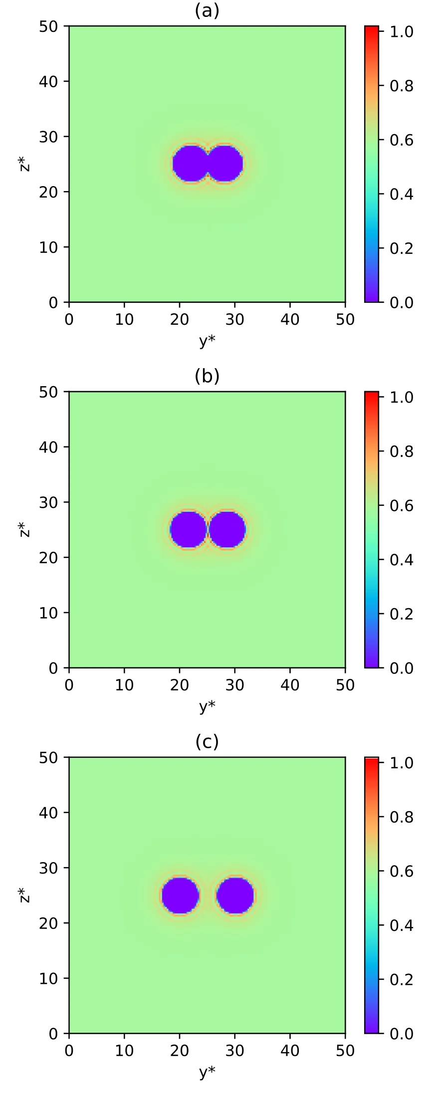
Figure 2.Density profiles of small spheres around two big spheres(a global view).(a)h*=0.0 when two big spheres touch each other.In this case,there is the largest overlap between two excluded volumes of big spheres and the total excluded volume reaches a minimum.The two central spherical regions are the excluded space of two big spheres.The density of the small spheres far away from the two big spheres is approximately equal to the bulk density.(b)h*=1.0 when the excluded volumes of two big spheres touch each other and the total excluded volume reaches a maximum.Also, the surface distance of the two big spheres is precisely allowed to contain one small sphere.(c) h*=4.0 when two big spheres are far apart and there is no overlap of the excluded volumes of the two big spheres.
3.3.Depletion potential and depletion force
Once the grand potential of a system is obtained by DFT,the depletion potential can be calculated using equation (17).When h*is large enough, Ω is approximated as the limiting value Ω(∞).We fit the data of the depletion potential by a 3-order spline curve.The spline interpolation uses a special type of piecewise polynomial called a spline as the interpolant.That is, instead of fitting a single, high-degree polynomial to all of the values at once, spline interpolation fits a low-degree polynomial to small subsets of the values.Spline interpolation is often preferred over polynomial interpolation because the interpolation error can be made small.According to equation(18),after we get the fitted curve of the depletion potential, the derivative of the depletion potential is taken to obtain the corresponding depletion force.In our implementation of DFT,we alter the parametersand T*to see how these parameters affect the depletion potential and depletion force.When one parameter is altered, the other parameters are fixed.For a definite value of a parameter, we vary the value of h*to perform a set of computations.Finally,we obtain the curve of the depletion potential and the corresponding depletion force with respect to h*.
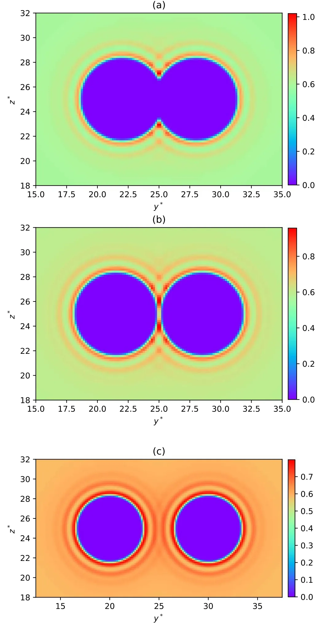
Figure 3.Density profiles of small spheres around two big spheres(a local view).(a) h*=0.0 when two big spheres touch each other.Here, there is the largest overlap between two excluded volumes of big spheres and the total excluded volume reaches a minimum.The central two spherical regions are the excluded space of two big spheres.The density of the small spheres far away from the two big spheres is approximately equal to the bulk density.(b)h*=1.0 when the excluded volumes of two big spheres touch each other and the total excluded volume reaches a maximum.Also, the surface distance of the two big spheres is precisely allowed to contain one small sphere.(c) h*=4.0 when two big spheres are far apart and there is no overlap of the excluded volumes of the two big spheres.

Figure 4.(a)The depletion potential of two big spheres immersed in a suspension of small spheres.Here,is varied from 1.0 to 7.0 with=2.0unchanged in all cases.The dots and other marks are data calculated using DFT, and the lines are fitted curves by 3-order spline interpolation.(b) The depletion force corresponding to the depletion potential in figure 4(a) by taking the derivatives of the depletion potential curves.
According to equation (19), we can alter the crossinteraction parameters ε*and σ*by changing the values ofand.Firstly,is varied from 1.0 to 7.0 with= 6.0,ρ* = 0.6,T* =2.0unchanged in all cases.We do not setto be smaller than one because a too smallmakes the depletion effect not obvious, which can be seen in the following analysis.The resultant depletion potentials and depletion forces are shown in figure 4.Overall, the largerresults in the larger depletion potential and depletion force.Also, except for in= 1.0, W(h*) is monotonously decreasing.In figure 4(b) we see that depletion forces are repulsive,except for= 1.0;that attractive part exists when h*is very small.The repulsive forces are caused by the unbalanced pressure exerted by small spheres between two big spheres and that between big spheres and borders.The narrow space between two big spheres enhances the collision of small spheres and the local pressure, which cannot be counteracted by the pressure from small spheres near borders,thus making the depletion forces repulsive.Note that the LJ potential equation (9) has the minimum −ε at r=21/6σ,hence the energy parameter ε in the LJ potential measures the depth of the attractive potential well.The smaller the energy parameter,the shallower the attractive well.The smaller value ofindicates the smaller cross-interaction parameter ε.Therefore, the interaction exerted on small spheres by big spheres includes less attraction and is primarily repulsion stemming from the hard-core, which contributes less to the local aggregation of small spheres around big spheres.Consequently, there is less local pressure imposed by small spheres on big spheres, resulting in less depletion potential and depletion force.The attractive force in contact when= 1.0is possible because the shallow attractive well of interaction between big and small spheres traps few small spheres in the narrow space between two big spheres, thus producing little pressure on big spheres, which is lower than the pressure on big spheres from outer small spheres.When h*is large enough,the depletion potential and depletion force asymptotically approach zero,because the pressure exerted by small spheres between two big spheres is counteracted by that between big spheres and borders.The depletion forces exhibit remarkable repulsive barriers and there is no oscillating behavior.These features of depletion potential and depletion force are obviously different from those of hard-sphere systems [46, 58, 80].In hard-sphere systems, the depletion potential typically has a negative contact value, and monotonously increases to positive.Meanwhile, it oscillates around zero and finally asymptotically approaches zero.The corresponding depletion force also displays a negative contact value and exhibits a repulsive barrier, then oscillates around zero with an asymptotic decay of amplitude.Such differences are primarily attributed to the difference in the interaction potential.As for the consequent repulsive forces in contact instead of attractive ones, it is related to the attractive part of the interaction potential[50],the bulk density of small spheres and temperature [81, 82].What is notable is that the extreme points of all the curves are approximately h*=1.0 (also observed in binary hard-sphere mixtures [45]), which corresponds to the physical scenario where the gap between two big spheres can precisely contain one small sphere and there is precisely no overlap of the excluded volume of big spheres:namely, the excluded volume reaches a maximum.In this case, the free space of small spheres is reduced to the minimum.Hence, there is the highest local pressure imposed by small spheres on big spheres and the depletion forces reach maximums.We discover that the contact value of W(h*) and F(h*) as well as the peak of F(h*) increase asincreases.This is because the deeper potential well attracts more small spheres between big spheres and these small spheres form layers that prevent big spheres from getting closer, thus causing a higher repulsive barrier.The attraction interaction of colloid–polymer and polymer–polymer both play a role in the accumulation of polymers around colloids [55].
Likewe changeranging from 4.0 to 10.0 with= 4.0,ρ* = 0.6,T* =2.0unchanged in all cases to obtain a set of depletion potentials and depletion forces and show them in figure 5.The reason that we do not choose a smallis that a too small size ratio of big and small spheres tends to cause a less prominent depletion effect,which will be shown in the following analysis.The overall results in figure 5 are similar to the situations in figure 4.In figure 5(a),the depletion potentials for all the parameters monotonously decrease.In figure 5(b), the depletion forces are mainly repulsive,except when= 4.0and 5.0 at the contact of two big spheres.Whenis increased,both the depletion potential and depletion force are enlarged and, in particular, the peak values of the depletion force also increase, indicating that a larger size ratio between big and small spheres can enhance the depletion effect.In the LJ potential equation (9), the length parameter σ is the zero-value point and also decides the minimum point.Thus, σ determines the interaction range of the LJ potential.The larger value of σ renders big spheres able to attract more small spheres to aggregate around big spheres, thus causing more local pressure on big spheres.Based on this excluded volume mechanism, the depletion effect tends to be enlarged.Once again,the peak values of the depletion force all appear when h*≈1.0.That is, when the total excluded volume of two big spheres reaches the maximum and the gap between two big spheres is only allowed to contain one small sphere.This is physically conceivable.

Figure 5.(a)The depletion potential of two big spheres immersed in a suspension of small spheres.Here,is varied from 4.0 to 10.0 with = 4.0, ρ* = 0.6, T * =2.0unchanged in all cases.The dots and other marks are data calculated using DFT, and the lines are fitted curves by 3-order spline interpolation.(b) The depletion force corresponding to the depletion potential in figure 5(a) by taking the derivatives of the depletion potential curves.
In the previous two scenarios, we set the bulk density ρ*=0.6.This is a relatively high density, and we would like to investigate the behavior of the depletion potential and depletion force in low bulk densities.Hence, we change the values of the bulk density ρ*from 0.1 to 0.6 withunchanged to obtain a set of depletion potentials and depletion forces.The results are displayed in figure 6.As ρ*increases,the contact value of the depletion potential and the peak value of the depletion force correspondingly increase, which is the same as the previous results for variedand.Nevertheless, for ρ*≤0.4,W(h*)is not monotonous and attractive wells of depletion forces exist.These characteristics exhibited by the depletion force are concerned with the density profile of small spheres between two big spheres.When the bulk density is high,there are more small spheres involved in forming dense layers in the narrow gap between big spheres, causing high local pressure and prohibiting big spheres from approaching each other, thus resulting in repulsive forces between big spheres.Moreover, the higher the bulk density, the higher the consequent repulsive barrier of the depletion force.However,for a relatively low bulk density, when the distance of the big spheres gets larger(for example,h*≈3 in figure 6),the layers between big spheres formed by fewer small spheres is less dense,which hardly counteracts the outer pressure exerted by the surrounding small spheres.Therefore, the depletion mechanism tends to render an effective attraction between two big spheres.This is meaningful for application to chemical processes and biological systems because we can vary the bulk density to change the features of the depletion forces.

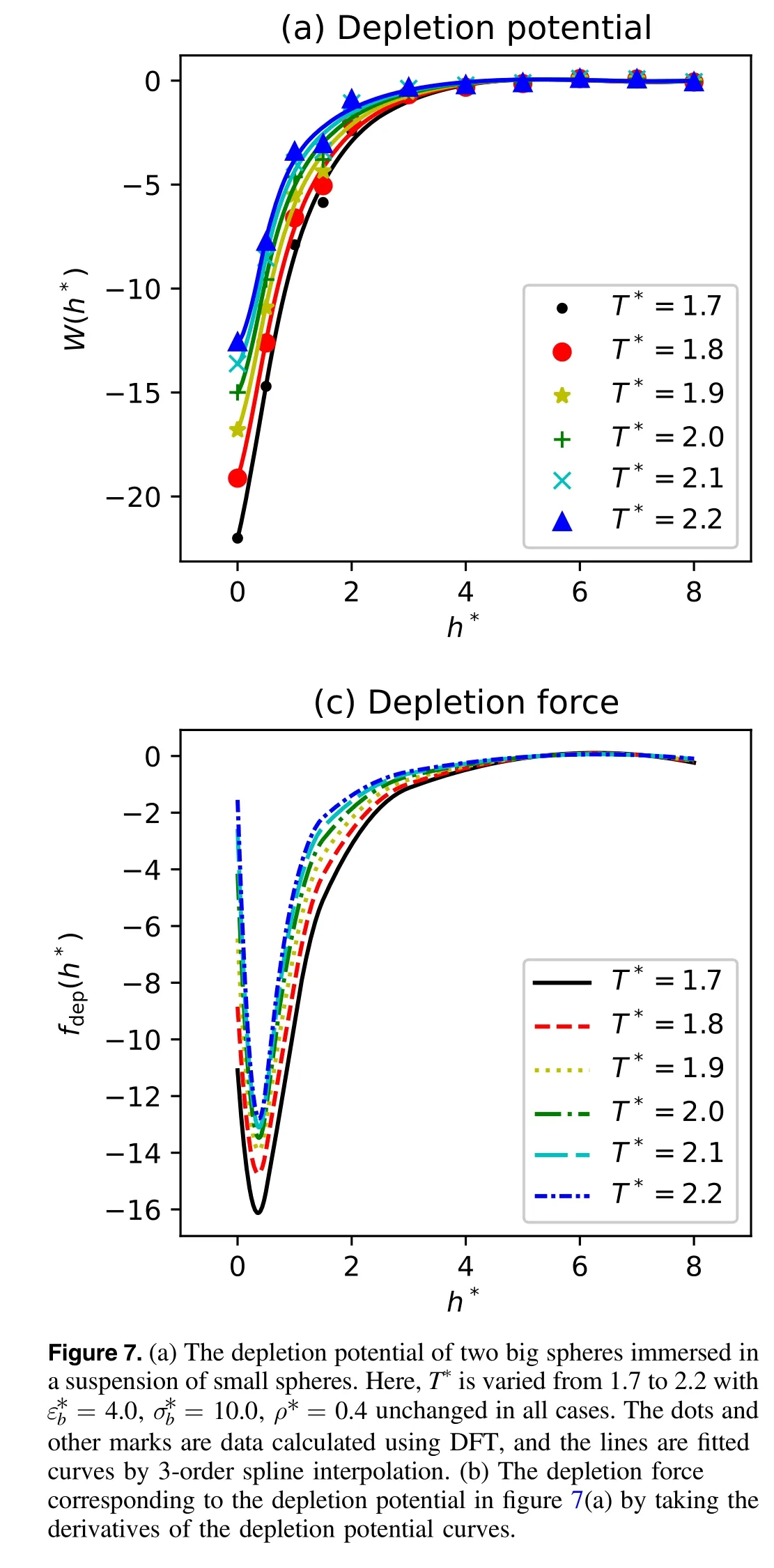
Next, we would like to determine the influences of the temperature of a system on the depletion potential and depletion force, especially whenis large and the bulk density is low, because the depletion effect will be enlarged and more features will be exhibited.Here, T*is varied from 1.7 to 2.2 with= 4.0,= 10.0,ρ* =0.4unchanged in all cases.The results of the depletion potentials and depletion forces are displayed in figure 7.The results are quite different from what those we found before.The remarkable difference in depletion potentials is the overall increasing tendency, and the corresponding depletion forces are primarily attractive.Notably, at h*≈0.5 there are sharp valleys in the depletion forces.It is conceivable that such differences are mainly due to the combined effect of an enlargednd diminished bulk density.As the discussion above reveals, a largetends to enhance the depletion effect of big spheres and low bulk density is prone to contribute to attraction between big spheres.The whole effect is the enhancement of the attraction effect.Besides, note that the minimum of the depletion force monotonously increases with respect to temperature, actually meaning the progressively diminished attractive force.This is possibly because the higher temperature endows larger kinetic energy of small spheres, making it easier for them to escape the bound region around big spheres, and thus leads to the decreased local pressure from the outer small spheres.What puzzles us is the appearance of minimums of depletion forces at h*≈0.5.When h*≈0.5,the geometric structure is special from the view of the excluded volumes of two big spheres.That is, one of the big spheres precisely contacts with the excluded volume of another big sphere.This configuration may have some influence on the depletion mechanism, but it needs further confirmation in later research.
4.Summary and conclusions
The depletion effect in the solute–solvent mixtures with the solute–solvent interaction modeled as hard-core and the solvent–solvent interaction modeled as a combination of hard-core and soft attraction have been investigated;however,the depletion interaction in the colloid–polymer system with all interaction considered as the LJ potential has not been studied.In this article,we implement CDFT to investigate the density profiles of polymers, and depletion interaction between colloids in LJ binary mixtures.The density profiles of polymers are regular: polymers approximately form concentric circles around colloids and, moreover, peaks and oscillations can be observed.We find whether the depletion force is attractive or repulsive depends on the bulk density of the polymer to a large extent.For high bulk densities the depletion potential is predominantly repulsive and no oscillation can be observed, in contrast to typical behavior of an attractive potential at short range, a remarkable repulsive barrier and oscillation at long range observed in hard-sphere binary mixtures.However,the depletion force displays both a repulsive barrier and an attractive well when the bulk density is small(typically less than 0.5)and the size ratio between the colloid and polymer is relatively small,in which the attractive well for larger distances of colloids is possibly related to the less dominant packing effect of polymers segregating between colloids.Moreover,low bulk density combined with a largecan cause the depletion force to be attractive and to exhibit a sharp attractive well.The repulsive or attractive behavior of the depletion force mainly comes from the unbalanced local pressure on colloids exerted by polymers between colloids and that between colloids and borders.The values ofand the bulk density of polymers can affect the repulsive barrier when the bulk density is high,and larger values of these parameters tend to heighten the repulsive effect.For attractive force in a low bulk density situation, a higher temperature tends to suppress the attractive effect and lower the depth of the attractive well.The significant feature of depletion forces is that the peaks of repulsive barriers all correspond to when the surface-to-surface distance of two colloids is approximately the diameter of a polymer molecule,indicating the important role played by the excluded volume mechanism in depletion phenomena.Distinctively, the attractive wells for low densities correspond to approximately half of the diameter of a polymer molecule,which may imply the significance of this special geometric configuration.While this study is helpful in that it further clarifies the mechanism of depletion interaction in colloid–polymer mixtures, more research is needed to understand the influences of factors like the geometric configuration of a system and the potential relations of the depletion effect with entropy and enthalpy.
Acknowledgments
We thank Shuangliang Zhao for helpful discussion and his valuable comments on the manuscript.This work was supported by the National Natural Science Foundation of China(Grant No.11504384)and the Fund of State Key Laboratory of Multiphase Complex Systems (No.MPCS-2017-A-04).The authors acknowledge HPC Cluster of ITP-CAS for supplying computation resources.
 Communications in Theoretical Physics2022年3期
- Communications in Theoretical Physics的其它文章
- Dynamics of mixed lump-soliton for an extended (2+1)-dimensional asymmetric Nizhnik-Novikov-Veselov equation
- Representation of the coherent state for a beam splitter operator and its applications
- Entanglement witnesses of four-qubit tripartite separable quantum states*
- From wave-particle duality to wave-particlemixedness triality: an uncertainty approach
- Photon subtraction-based continuousvariable measurement-device-independent quantum key distribution with discrete modulation over a fiber-to-water channel
- Enhancement of feasibility of macroscopic quantum superposition state with the quantum Rabi-Stark model