Electron beam modeling and analyses of the electric field distribution and space charge effect

Yueling Jiang(蒋越凌) and Quanlin Dong(董全林)

School of Instrumentation and Optoelectronic Engineering,Beihang University,Beijing,China

Keywords: electron beam,electric field distribution,space charge effect

1. Introduction

The electron beam technology plays a vital role in various industrial processes,especially in the highly propulsive fields of aeronautics and astronautics. The electron beam quality parameters, as the core indicators of the electron beam characteristics,decisively influence the outcome of the electron beam application.[1]As the charged electrons form a beam,the beam tends to diffuse as a result of interactions between particles. It is necessary to analyze the electric and magnetic field intensity generated by the electron beam to study the space charge effect(SCE).

There are mainly two ways to study the diffusion of charged particle beams caused by the SCE. The first one is to predict the trajectory of a ray with a differential equation known as envelope equation or ray equation. In 2000,Raghebet al.,using findings on a beam with a uniform current density distribution obtained by Zhigarev,[2]described the derivation of the formula for the envelope prediction. In 2011,Takahashi applied the same equation in the method of average space charge effect when comparing different methods of predicting electron beam diffusion,[3]whereas in 2009, the book edited by Orloff introduced a complete version of the ray equation.It uses multiple series in the expression of corresponding envelope equations of the electric field intensity under various current density distributions[4]

whereris the radius of the tracked ray,r0is a characteristic measure of the beam radius,zis the coordinate of the axis parallel to propagation speed, anda,b,care determined by the current distribution. The envelope equation tracks only one ray,and consider its radius as the width of the beam when predicting the beam width. As a result, the envelope can have a overly small minimum width and the tracked ray never crosses the axis. While in reality,the envelope of a beam usually consists of multiple rays and an outer ray usually crosses the axis.Therefore, such an equation may not be effective for width prediction.

The second way is to directly study the electric and magnetic intensity generated by a beam and conduct numerical simulations. Currently,there are some plain methods for electric field calculation.[5,6]For instance,Chauvin of CERN studied the electric and magnetic fields excited by the charged particle beam,applying Gauss’law,the numerical calculation of the cross-sectional electric field intensity generated by the particle beam was performed, and the analytical expressions under several standard distributions were derived.[6]The same author also studied space charge expansion under specific conditions.

Chauvin’s derivation is based on a uniform and infinite long beam,and the results from such overly ideal model may have neglected measurable factors.We intend to fully consider the electron beam to deduce the exact results of the electric field distribution and then simulate the beam propagation.

The remainder of this paper is organized as follows. Section 2 introduces the electron beam model. The simulations and their results are discussed in Section 3. Finally,Section 4 concludes the paper.

2. Electron beam model

Based on the current experimental results and theoretical research,the following assumptions can be made for the electron beam. Firstly, the electron beam has a particular initial cross-sectional area and a corresponding convergence or divergence angle. This angle is very small,generally at the milliradian level,and can be neglected when calculating the field intensity. Secondly, as all electrons are accelerated with the same voltage and the lateral velocity is insignificant, we can consider that all electrons have the same axial velocity after acceleration. Considering any particular section in the middle of the electron beam,as the front and rear parts of the electron beam have similar strengths of forces to the section, and the electric field force generated by the moving electrons in the longitudinal direction is small, it can be considered that the axial velocity of the electrons is constant. Thirdly,the current density follows a specific distribution on the cross-section and poses a rotational symmetry. Each concentric circle on the cross-section follows the same current density, and the electrons are continuously distributed in space.[2,7–9]

2.1. Electric field distribution

Let us consider two particles with identical charges,q. If the particles are at rest,the Coulomb force exerts a repulsion,and if the particles travel with a velocityvz,they represent two parallel currentsI=qv,which attract each other owing to the effect of their magnetic fields. Further, let us consider a particle in an unbonded beam of particles with a circular crosssection. Coulomb repulsion pushes the particle outward. The induced force is zero at the beam center and varies along the radius of the beam. The magnetic force is radial and attractive for the test particle in a traveling beam, retarding the beam spread.

According to electrodynamics, the electric and magnetic fields excited by a moving electron with uniform velocityvin space are[10,11]

whereRis the vector from the source point to the field point,θis the angle betweenRand the electron velocity vector,ε0is the vacuum dielectric constant,eis the charge of the electron,cis the speed of light,EandBare perpendicular to each other,andBisv/c2timesE. When sinθ=1, only the particles on the cross-section are considered,whereRis perpendicular to the electron velocity vector. The following equation is obtained by integrating as in Fig.1,which shows the electric field excited by the cross-section at a distancerfrom the center of the circle:

vzis the axial velocity,Ris the radius of the beam, and the electric field vector points to the center of the circle from the field point. Note that Eq. (3) is only a preliminary formula,and its dimensions are not strictly specified.

Fig.1. Schematic of cross-sectional integration.

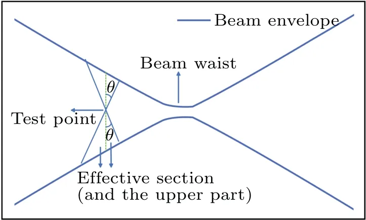
Fig.2. Schematic of effective section.

Next, we expand the scope of the equation to space and replace the field strength generated by a single point in Eq.(3)with the electric field intensity generated by all electrons,calculated for a point on the cross-section at a fixed axial distance, and then perform the integral operation to obtain the expression for the electric field intensity generated by the corresponding electric charge in space. Equation (1) shows that the intensity of the electric field generated by moving electrons decreases asθdecreases,and reaches a maximum at 90°,that is, an electron generates the maximum field intensity on the cross-section where it is located. The field strength decreases with a decrease in the angle,and it should be neglected when the electric field strength reaches a negligible level. The actual angle depends on specific conditions. Suppose the angle isθ,the effective section for a test point shown in Fig. 2 is a fanshaped zone with the axis of symmetry parallel with the axis at the center of the circle,Ris the symmetry axis,andθis the half-angle. The electric field generated by the electrons in the zone above is considered. Because the area where the error may occur is far from the test point,it can be assumed that the axial characteristics of the electron beam do not change in the area. The component of the electric field intensity generated by the corresponding electrons at the cross-sectional point in the longitudinal direction can be calculated as follows:

Equations(6)and(7)are the complete formulae and also applicable to other charged particle beams.Bisvz/c2times ofEand the direction is perpendicular toE. Equation(6)gives the electric field generated by the averaged space charge effect,and its counterpart is the discrete space charge effect, that is,the mutual influence of two close electrons. For charged particle beams,the space charge effect dominates the diffusion of the beam when the current density is large. According to the Lorentz force formula, the force hindering the spread of the electron beam isv2z/c2times the electric field force.

2.2. Comprehension and verification

A Gaussian distribution is a common form of the beam current density distribution. For a circular Gaussian distribution,the current density is given by[12]

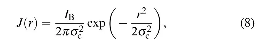
whereIBis the beam current,andσcis the standard deviation of the Gaussian beam. In the Gaussian distribution, the area within the horizontal axis interval (μ-2.58σ,μ+2.58σ) is 99%,and thus,2.58σ=R,whereRis the characteristic beam radius. The form below can be found by calculating

Equation (10) is the analytical expression under a Gaussian distribution, and the forms based on other distributions can also be obtained. The value of the second part of the expression in Eq.(6)is always zero,hence,it is known that the electrons outside the radius of the test point under the rotationally symmetric current density do not affect the electric field, and thus conform to Gaussian law. Therefore,the final versions of Eqs.(6)and(7)are

whereρ(r′)is the charge density atr′,ρ0gis the charge density at the center of the beam,ε0is the vacuum dielectric constant,andσis the standard deviation of the Gaussian distribution.The calculation result shows the conformity of Eqs. (10) and(14), except for the definite integral ofθin Eq. (10), which verifies the correctness of Eq.(10). Meanwhile,the deduction method used in this study better reveals the inherent characteristics of the beam. The variableθintroduced makes it feasible to determine the range of the considered beam according to actual conditions such as axial speed,which reduces the errors caused by different beam current conditions far from the test point, especially a different current distribution at a distantzcoordinate.

3. Simulations and analyses

3.1. Basis

According to the equations and experimental results,SCE is significant when the current of the beam is large. Therefore,to study the characteristics of SCE,it is best to take a typical high current beam as an example. This simulation is mainly based on the experimental and calculation results obtained by Kolevaet al.[8]Through experiments,they measured the current density of an electron beam at 320 mm, 245 mm, and 170 mm from the focusing coil, where 320 mm is the focal plane position of the electron beam, and the current density change from 170 mm to 320 mm shows a focusing process.The electron beam current was 40 mA, the acceleration voltage was 60 kV, and the power was 2.4 kW. Then, they used a Monte–Carlo simulation to calculate the current density distribution in the three sections. The distributions at 320 mm,245 mm,and 170 mm are as follows:

The units are mA/mm2. For the Gaussian distribution of the current density,the beam radius corresponds to the distribution. If we letR=2.58σ,the radii of the beams above are 3.030 mm, 1.548 mm, and 0.407 mm, respectively. The current,voltage and radii mentioned above were used in the simulation. The axial velocity of the electron obtained through the relativistic kinetic energy formula was 1.33×108m/s at a voltage of 60 kV.

3.2. Simulation of electric field distribution

Because there is currently no pattern to determineθin Eq.(12), andθmust be less thanπ/2, with the integral ofθbeing less than 1, we let 2/πreplace the definite integral in Eq. (12). Based on the previous formula and data, the current density distributions and corresponding electric field intensity distributions on the cross-section are obtained as shown in Fig.3.

Figure 3 shows the current density distributions and field intensity distributions under three radii, respectively, where the third radius is slightly less than 0.4 mm. The blue curves represent the current density distributions, corresponding to the leftY-axis, and the red curves are the electric field distributions, corresponding to the rightY-axis. From Fig. 3, it is clear that the maximum current density increases rapidly as the beam radius decreases, and the maximum current density is inversely proportional to the square of the radius from the Gaussian distribution expression. Similarly,the maximum electric field intensity increases rapidly as the beam radius decreases,albeit not as fast.

Fig.3. Distributions of current density and electric field intensity with different widths.

The following rules can be summarized from the analytical formula and simulation results. Firstly,the field is nonlinear inside the beam and varies according to 1/rwhen far from the beam (severalσc). Secondly, the field intensity is zero at the center of the beam, increases first, and then decreases as the distance increases. The field intensity is proportional to the current when the beam radius is constant. When the current is constant,the maximum field intensity increases with a decrease in the radius,and the field intensity is inversely proportional to the electron axial speed. Thirdly, the maximum field intensity appears at 1.585σcfrom the center of the circle,that is,0.613R.

3.3. Simulation of SCE

The initial conditions of this simulation are as follows:the accelerating voltage is 60 kV,total current is 40 mA,initial width of the beam is 3.030 mm, and theoretical focal length is 150 mm (which means the beam focuses after traveling 150 mm from the initial plane without SCE), and the aberrations can be ignored under such conditions. The current density is considered to follow the Gaussian distribution, and all rays share the same constant axial velocity. In this simulation,100 rays inside the beam are tracked during their travel.

In Fig. 4, the rays or light paths are marked by different shades of gray according to their initial distance from the center to characterize the current density. The larger the number,the larger the initialxcoordinate, and the smaller the current density. According to the simulation, thezcoordinate of the actual focal plane is approximately 165 mm with a minimal beam width of 0.162 mm. The neglecting of off-axis focusing makes the simulated minimal width smaller than the experimental width. The beam can be viewed as a combination of three parts: The first part exists from 0 mm to 144.6 mm,the second part exists from 144.6 mm to 172.9 mm,and the rest of the beam constitutes the last part.Ray 100,with the largest initialxcoordinate,forms the beam envelope of the first and third parts, whereas multiple rays form the envelope of the second part, which means that the laminar flow condition stops before the second part. The comparison of characteristic widths at differentz-coordinates of the simulation and experiment as the basis whenR=2.58σis given in Table 1.

Fig.4. Beam propagation and ray tracking.

Table 1. Comparison of experimental and simulation widths.

The comparison shows that the simulation data match the experiment well,which proves the ray tracking method effective for beam width prediction. The widths atz=150 mm show a measurable difference,which can be explained by several reasons. Firstly, the phenomenon of off-axis focusing of the beam is not considered in this simulation because it can not be accurately simulated based on the existing results. Off-axis focusing occurs because of electrons with a velocity not parallel to axis,theoretically,off-axis focusing lets a beam focus on a disc instead of a point on the focusing plane and it mainly affects the beam width near the focusing plane, this explains the inconsiderable difference between data atz=75 mm. The estimating of exact effect of off-axis focusing is difficult because it can not be directly measured in an experiment. Under given condition,an estimate equation can be given as

whereWminis the actual minimal beam width,WSCis the minimal width when off-axis focusing is not considered, andWois the off-axis focusing height. According to Eq.(15),the offaxis focusing height in this case is about 0.2 mm. Secondly,the existence of statistical Coulomb interactions among discrete electrons. Though Takahashi’s research shows that discrete interactions between electrons are not dominant when the current is high,[3]they may still have a certain contribution. Thirdly, the experimental parameters and data, as well as the simulation data,may contain errors. Above all,off-axis focusing is the main contributor in this case.

To study the flow in detail, thex-coordinates of all rays during the entire propagation are shown in Fig.5,where thexcoordinates are represented by different colors,and the upper half of the beam is tracked. The four parts of the rays can be distinguished as shown in Fig. 5. The first part is marked by the smallest number and sticks to the axis where the electric field intensity is insignificant. Obviously, positivexcoordinates characterize the rays in the second part at the end of the propagation. The rays of the third part end up near the axis.The rays of the fourth part travel from the top of the beam to the bottom.

Fig.5. The x coordinates of all rays on different z coordinates.

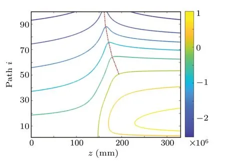
Fig.6. Contour of radial velocities of all rays.

Further, the contour of the radial velocities of all rays is shown in Fig.6,where colors of different contour lines show their radial velocities. A positive value denotes upward motion,whereas a negative value denotes downward motion. All rays move downward initially as we track the upper half of the beam. According to Fig.6,more than 50%of the rays fail to cross the axis and all of them are marked with a smaller number than the rays that cross over. The red dotted line shown in Fig. 6 indicates the “ridge” where the rays cross the axis. A similarity is noticed between SCE and spherical aberration as the upper rays crossed the axis earlier than the lower rays.

The simulation of SCE provides a method for beam width prediction, hence the possible maximum resolution of the beam is given. The obtained data clearly reveal the flow pattern of the beam as the trajectory and radial speed of every ray are displayed,and an in-depth investigation into such data can be applicable for optics design optimization. Further, a comprehensive analysis with SCE, abberations, off-axis focusing etc. involved is feasible based on data obtained in corresponding simulation applying the ray tracking method.

4. Conclusions

A model for analyzing the electron beam propagation is proposed, and the corresponding electric and magnetic field integral expressions are obtained. The analytical equation under the Gaussian distribution is obtained and verified with the CERN results. Simulations are conducted, and the results are analyzed. The cross-sectional electric field distribution is mainly affected by the electron beam emission current,current density distribution,and electron beam propagation speed. For the same distribution, a stronger current and more intense electric field of the electron beam cross-section would cause the electron beam to expand more easily. The value ofθin the definite integral is affected by multiple factors simultaneously,the impacts of which require careful consideration.Tracked rays show the flow pattern inside the beam and envelope, which consists of multiple rays. The comparison of simulation and experimental data shows a good match and proves the method used effective for beam width prediction and beam simulation. A similarity is observed between SCE and spherical aberration.

Acknowledgement

Project supported by CAST Innovation Fund(Grant No.CAST-BISEE2019-040).