
Fringe removal algorithms for atomic absorption images: A survey
2022-05-16 07:08GaoyiLei雷高益ChenchengTang唐陈成andYueyangZhai翟跃阳
Chinese Physics B 2022年5期
Gaoyi Lei(雷高益) Chencheng Tang(唐陈成) and Yueyang Zhai(翟跃阳)
1School of Instrumentation and Optoelectronic Engineering,Beihang University,Beijing 100191,China
2Quantum Sensing Center,Zhejiang Laboratory,Hangzhou 310000,China
3Research Institute of Frontier Science,Beihang University,Beijing 100191,China
Keywords: atomic absorption image,fringe removal,principal component analysis,deep learning
1. Introduction
Absorption imaging is an important technique for the precise measurement[1–3]and many-body quantum systems.[4–6]The absorption imaging technique passes a probe beam through the atomic cloud,and leaves a shadow in the transmitted beam.[7]This shadow contains the spatial distribution of the atomic cloud,and can be recorded by the CCD camera.[8,9]Optical density (OD) can be calculated from the atomic distribution,which is useful for quantum metrology,[10,11]phase transitions[12,13]or dimensional crossover.[14,15]To compute the OD of the absorption image, researchers can record the reference image shortly after the absorption image without the atoms, and do the logarithm subtraction with the absorption image.[16]This survey assigns this result as ODref. In practice,ODrefsuffers from the unwanted reflections which generate the stripes and Newton’s rings.
The dynamics of the beam light causes different residual fringe noises in the ODref. These fringe noises cause the problem to distinguish the atom distribution from the background. To improve the quality of the OD,the fringe removal algorithm analyzes the fringe pattern to eliminate the influence of the noises around the atom distribution. As Fig. 1 shows, the fringe removal algorithm searches the edge areas to compute the fringe patterns. The edge areas can be chosen as the reference images or the edge parts of the absorption images, which are filled with the fringe signals without atom information. Then the algorithm generates the ideal reference image,whose fringe pattern has been fitted with the test atom area. This fitness process of the fringe patterns provides the promise to remove the fringe signals thoroughly with the generated ideal reference image.
According to the feature extraction approaches, this survey classifies the fringe removal algorithms(e.g.,listed in Table 1) into two categories: the image-decomposition based methods[16–21]and the deep-learning based methods.[22]The image-decomposition based methods decompose the reference images or the edge areas (without atom information) to calculate the fringe basis set. The deep-learning based methods directly predict the ideal reference image with the masked atom area in a trained network. Ockeloenet al.computed the singular vectors of the fringe patterns with singular value decomposition (SVD) in a dataset of hundreds of absorption images.[19]Niuet al.proposed the optimized fringe removal algorithm(OFRA)to reduce the noise signal,and determined the fringe patterns by modifying conditional principal component analysis (PCA).[18]Nesset al.introduced the deep learning into the fringe removal research,and adopted a U-net model to predict the ideal reference image of the absorption image.[22]
These researches usually assigned the fringe removal algorithms with the absorption imaging systems,leaving the gap of interpreting the algorithm development. The aim of this survey is to review the fringe removal algorithms in the workflow level, and present the breakpoints of current fringe removal researches. We draw the workflows of the enhanced PCA (EPCA) method[16]and the U-net method[22]in Algorithm 1 and Algorithm 2, respectively. The former is a complex image-decomposition based method, and the latter is a novel deep-learning based method.Then we discuss the potential applications of generative adversarial network(GAN)and transfer learning for atomic fringe removal. Finally, we conduct fringe removal experiments on the absDL ultracold image dataset[22]and evaluate the performance with the peak signal noise rate (PSNR). Results suggest that the SVD method[19]outperforms other fringe removal algorithms, and the deeplearning based method is feasible.
The remainder of this paper is organized as follows. Section 2 presents the image-decomposition based methods, and Section 3 shows the deep-learning based methods. Experiments of the fringe removal algorithms are conducted in Section 4. And Section 5 concludes this survey.
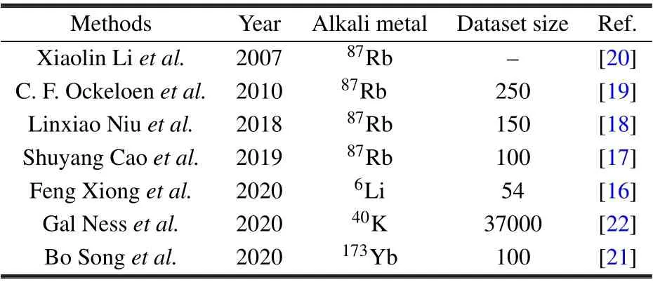
Table 1. Details of the fringe removal algorithms for atomic absorption images.

Fig.1. The flow chart of the fringe removal algorithms. Fringe patterns are extracted from the edge area(without the atom information),and are utilized to generate the ideal reference image of the atom area(with the atom information). These data samples are selected from the open-access absDL dataset.
2. Image-decomposition based methods
This section reviews the image-decomposition based methods in the process of the absorption images. The edge areas are decomposed into matrices multiplication, and the eigen-vectors are collected to build the fringe basis set. So we mark this kind of fringe removal algorithms as imagedecomposition based methods.
Assume there arenabsorption images andnrecorded reference images(ornedge area images),and the pixel number of these images ism. Firstly, we subtract the absorption images and the reference images with the background of dark exposure. Then the absorption images are stacked into the absorption matrixA(A ∈Rm×n),and the reference images are stacked into the reference matrixL(L ∈Rm×n). Suppose there exists a matrixA′,which excludes the atom information and has the same fringe structures with the absorption matrix. Then OD is calculated as following:

where the logarithm operation is implied in every element of the matrixAandA′.
We can regard the matrixLas an alternative of the ideal reference matrixA′, and assign the result as ODref. However, the dynamic difference of the imaging system causes residual fringe noises in the ODref. The aim of the imagedecomposition based methods is to calculate the fringe basis set from the train dataset, and reconstruct the ideal reference images of the absorption images. A classical workflow of the image-decomposition based methods would obtain the“mean image”matrix ˜L,by subtracting the reference matrixLwith its mean value. Then apply the singular value decomposition

whereUis the left singular vector,Σis the singular value matrix,andVis the right singular vector.
The left singular vectorUis utilized to build the fringe basis set, and the matrixAsubtracts its mean valueE(A), resulting in the mean absorption matrix ˜A. This classical workflow projects the ˜Ainto the fringe basis set, and adds the result withE(A)to generate the ideal reference matrixA′. The breakpoints of the image-decomposition based methods are mainly the processes of computing the vectorUand building the fringe basis set.
The SVD method calculates the singular vector of every column of the mean reference matrix ˜L, and uses all singular vectors to build the fringe basis set, without examining the importance of different singular vectors for fringe removal.[19]The optimized fringe removal algorithm(OFRA)method masks the atom area in the projection of matrix ˜A.Then the PCA technique is implied to search the principal components of the fringe patterns. The OFRA method is suggested to outperform the conditional PCA method in computing the physical parameters of the time-of-flight (TOF) images,by excluding the atom information in the reconstruction of the ideal reference images.[18]

Algorithm 1 The workflow of the EPCA method Input: The reference images L Input: The atom absorption images A Input: The dark background image G Output: The optical density OD Subtract L and A with G, obtaining ˜L and ˜A. Create an empty fringe basis set U.for i=1:EpochNum do ˜Lorigin= ˜L-mean(˜L);Initialization,L= ˜Lorigin for j=1:8 do LF)filter=GaussianFilter(LF =FourierTransform(L)(LF)LF)filter)Select the largest singular vector of Lfilter=InvesrFourier((Lfilter,uj filts=pinv(L·uj),pinv is the pseudo-inverse operation Fitting the dataset with uj,L=L-uj·filts·L end for Select the largest four singular vectors in {u1,...,u8},add them into U.Compute the largest singular vector of L,and add it into U.end for Project the ˜A into the fringe basis set U, and generate the ideal reference images A′Apply the logarithm operation and compute the optical density,OD=log(A)-log(A′)
The EPCA method applies Fourier transformation before decomposing ˜L.[16]˜Lis filtered with a two-dimensional bandpass filter in the position of highest pixel in the frequency domain. Filtered images are transformed back through the Fourier inverse transformation operation, with the real parts and imaginary parts. Real parts and imaginary parts are stacked to construct one filtered fringe pattern. Fitting this fringe pattern to dataset and repeat above steps to generate next filter fringe patter(as shown in Algorithm 1). The EPCA method computes 8 filtered fringe patterns and 1 normal fringe pattern in single epoch with 15 epochs in total,and deprecates the useless patterns with least squares fit.[16]
Songet al.considered the defect of ultracold imaging system and proposed a data augmentation method to extend the number of the fringe basis setF.[21]Data augmentation can enlarge the dataset size without acquiring extra samples. As the interference fringe presents in plane wave,a spatially shift in horizontal axis and vertical axis is designed to augment the original absorption image in this data augmentation method.Caoet al.recognized the physical sources of the fringe structures in time-of-flights images with the PCA method.[17]They pointed out that the main physical sources of the fringe noises in one-dimensional optical lattices are the position fluctuation,the atom number fluctuation,and the normal fluid fraction,and so on.
The image-decomposition based methods analyze the singular vector of the reference images,and reconstruct the ideal reference images of the absorption images with the fringe basis set. Though the breakpoints of the image-decomposition based methods are different,the fringe patterns are calculated as the fringe basis set in the matrix style.
3. Deep-learning based methods
This section reviews the deep-learning based fringe removal methods, and discusses the advanced deep learning techniques in the process of the absorption images. The deeplearning based methods learn the fringe patterns in the hidden states of the neural network,and provide an approximation of the ideal light distribution in the masked atom area.
3.1. The U-net method
The U-net method introduces the deep learning techniques and the image inpainting ideas into the fringe removal in absorption images.[22]The U-net method masks the atom area and transfer the fringe pattern extraction problem to the image restoration problem. The deep neural network adopted in this method is the U-net model,[23]which consists of the down-sample path, the up-sample path and the skipconnections between these two paths. The basic network layers in the U-net model are the convolution layer,the activation layer,the batch normalization(BN)layer,and so on.
The convolution layer implies the convolution filters on the input and computes the feature maps, whose dimension is the number of the convolution filters.[24]The convolution filters are often designed as 3×3 or 5×5 matrices. The calculation of the(i,j)-th pixel of the convolution layer is presented as Conv(i,j)=(xconv*ω)[i,j],(3)where thexconvis the input to the convolution layer,ωstands for the convolution filter,and*is the convolution operation.
As the data distribution shifts during the training of deep neural network, the batch norm (BN) layer is adopted to stabilize the data distribution during the training process of deep neural networks. The BN layer can make the network optimization smoothly such the gradients are more predictive and the network converge faster.[25]The equation of the BN layer is presented as following:

wherexBNis the input of the BN layer,μis the mean value ofxandσ2is the variance ofx.εis a small number to prevent the failure of the division.
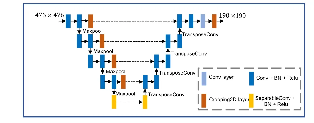
Fig.2. The network architecture of the U-net method. The size of the input is 476×476, and the size of the output is 190×190. The meaning of the blocks are present in the right box. “BN” is the batch normalization layer,“Maxpool” is the 2D max-pooling layer, and “TransposeConv” is the 2D transpose convolution layer.
The non-linear activation layer, rectified linear unit(ReLU),[26]is applied after the convolution layer and the BN layer in the U-net method. Other possible activation functions are sigmoid, leaky ReLU, tanh, and so on. The equation of ReLU is

wherexReluis the input of the ReLU function.
The workflow detail of the U-net method is shown in Algorithm 2. The U-net method transfers the atom images and the reference images into the 32-bit type,and crops their size into 476×476 pixels. The central area of the recorded images is masked with a circle of 190 pixel diameter to create an image restoration problem. A U-net architecture is implied to learn the masked images, and predicts the ideal light distribution around the atom area. As Fig.2 shows,the network architecture consists of 18 convolution layers,2 separable convolution layers,4 max-pooling layers,4 transpose convolution layers and 5 cropping layers. These 32 layers contains about 20×106parameters. The Adam optimizer with the learning rate of 5×10⁻⁶is applied to update the network parameters,and the batch size is 8. The objective function of the restoration problem in the U-net method is designed as the mean error loss function. Four cropping 2D layers cut the shape of data from the 476×476 (input) to the 190×190 (output), which forces the U-net model predict the information around the central area. Nesset al.suggested that the U-net method is robust to the variations of the working conditions through time.[22]
The U-net method introduces the novel image inpainting idea into the fringe removal researches,which extends the applications of the deep learning techniques in the process of the absorption images.The U-net method can learn the fringe patterns from massive data, and perform robust to the variations in the experimental conditions. However, the U-net method requires sufficient data to guarantee the performance. The implementation of the deep-learning based methods is more complex than the image-decomposition based methods, from the perspective of the basic modules and software platforms.The module layers of the U-net method are implemented in the Keras and tensorflow platform,[27]which are developed for the deep learning techniques.
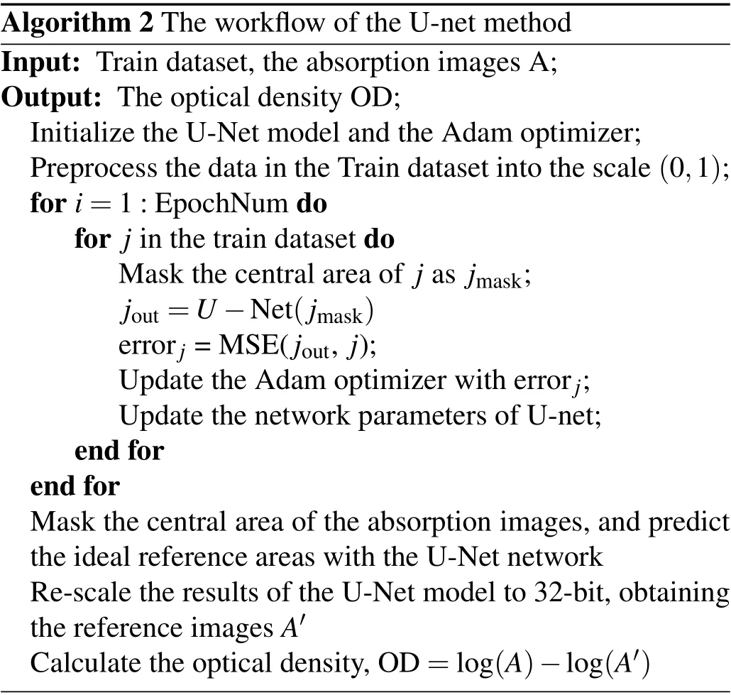
Algorithm 2 The workflow of the U-net method Input: Train dataset,the absorption images A;Output: The optical density OD;Initialize the U-Net model and the Adam optimizer;Preprocess the data in the Train dataset into the scale(0,1);for i=1:EpochNum do for j in the train dataset do Mask the central area of j as jmask;jout=U-Net(jmask)errorj =MSE(jout, j);Update the Adam optimizer with errorj;Update the network parameters of U-net;end for end for Mask the central area of the absorption images,and predict the ideal reference areas with the U-Net network Re-scale the results of the U-Net model to 32-bit,obtaining the reference images A′Calculate the optical density,OD=log(A)-log(A′)
3.2. GAN and transfer learning
This subsection discusses the potential applications of GAN and transfer learning. Though Nesset al.succeeded to imply the U-net method and restore the masked absorption images,[22]the U-net model often suffers from the boundary artifacts and blurry textures in image inpainting.[28]GAN is a popular technique to generate high-quality restoration samples, and has been applied in the inpainting of medical images,[29]face images,[30]and scene images.[31]
A common module of GAN consists of a generator and a discriminator. The generator learns the distribution of the actual dataset and produces the generated samples. And the discriminator distinguishes the generated samples from the actual data. Thus,the generator and the discriminator play a minmax game, training the networks in an adversarial approach.[32]In order to enhance the divergence of GAN, the Wasserstein GAN(WGAN)is proposed to imply the Lipschitz restriction and measure the distance of the data distributions with the Wasserstein distance.[33]Yuet al.combined the WGAN and the contextual attention to capture the global information and generate high-quality restoration samples.[28]This contextual WGAN method is potential to solve the ineffectiveness problem of the U-net method,with the loss function on the global areas and the masked areas.
Current fringe removal algorithms explore the impact of the fringe removal algorithms on the physical system, without extending the algorithms across different physical systems.Assume there are two absorption imaging systems with different alkali metal,the source system and the target system. Current fringe removal algorithms require sufficient recorded data both in the source system and the target system, and the extracted fringe basis set in the source system is not considered for the target system.Transfer learning can conduct the knowledge transformation across different domains.[34]Panet al.proposed a transfer learning method named transfer component analysis(TCA),mapping the source domain and the target domain to a reproducing kernel Hilbert space to learn the transfer components.[35]TCA is potential to transfer the fringe basis set from the source system to the target system.
The U-net method introduces the idea of the image inpainting to the fringe removal research. However, the U-net method suffers from the ineffectiveness of the convolution layers,and the acquired fringe patterns can not be utilized across different physical systems. GAN and transfer learning are popular techniques in computer vision techniques, which can be implied to extend the fringe removal researches.
4. Experiments
This section conducts experiments of four fringe removal algorithms on the absDL dataset, to present the performance and the realization of fringe removal algorithms. The four fringe removal algorithms shown in this section are the SVD method,[19]the OFRA method,[18]the EPCA method,[16]and the U-net method.[22]
4.1. Dataset and the PSNR evaluation
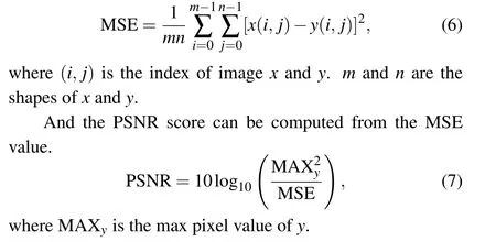
The atom absorption images and the reference images utilized in this section are selected from the absDL ultracold absorption images dataset. Nesset al.conducted experiments with a quantum degenerate Fermi gas of40K atoms,and published the absDL dataset with 37000 reference images and 720 atom absorption images.[22]The images in the absDL dataset are taken with a laser at the wavelength of~766.7 nm and the line width of 100 kHz. We select 100 atom absorption images as the test set, and 250 reference images for the calculation of fringe patterns in the image decomposition methods. The number of the reference images required by the image decomposition methods is determined according to the description of the original research articles. Then we introduce the peak signal noise rate(PSNR)as the quality evaluation in our experiments. We mark the reference image asy,and the reconstruction image asx. The fundamental mean square error (MSE)value is calculated as following:
4.2. Results
This subsection presents the OD results of the four fringe removal algorithms. The variable parameters and settings of the experimented fringe removal algorithms are determined according to their original researches. Results show that the SVD method with 250 recorded images achieves best performance,and the U-net method accomplishes the fringe removal in a novel approach.
The PSNR evaluation results are listed in Table 2,where the SVD method achieves the score of 32.4795. The U-net method outperforms the OFRA method and the EPCA method with the score of 32.2564. Figure 3 shows the OD results of the fringe removal algorithms on a random sample from the absDL dataset. The top row of Fig. 3 presents the reference image and the generated ideal reference images of the four fringe removal algorithms. The bottom row of Fig. 3 shows the OD results which also suggest that the SVD method performs well.It is observed that the atom area in the result of the EPCA method is a little blurry compared with other imagedecomposition based methods, which may be caused by the information loss in the process of the Gaussian filter. The four corners of the OD result of the U-net method are near black,because the areas in the four corners are unmasked and the network only predicts the circle masked area.
The idea of the image-decomposition methods is to compute the fringe basis set, and project the absorption images into this set to removal residual fringe structures. The SVD method,the OFRA method and the EPCA method design different strategies of extracting the fringe basis set, in the process of computing the singular vectors. However, the results in our experiments suggest that the simple SVD method can achieve outstanding performance with proper parameters and adequate train set. The success of the U-net method guarantees the future applications of the deep learning techniques,whose developments are fast in the computer vision area.
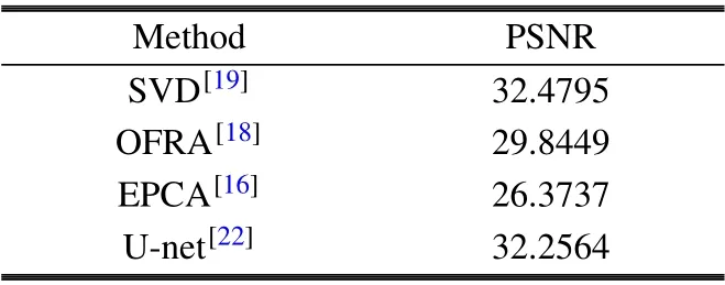
Table 2. The mean PSNR evaulation result.
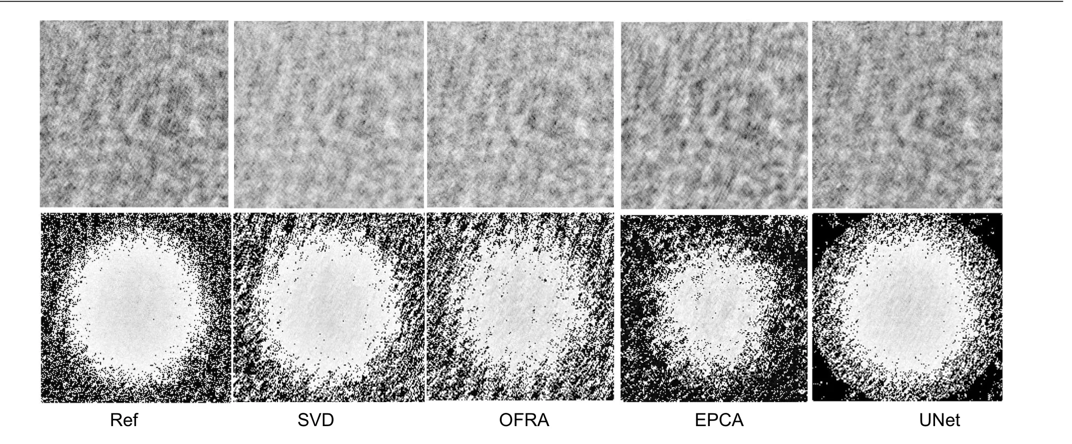
Fig.3. The OD results of the reference image and the fringe removal algorithms on one absorption sample. The top row shows the reference image and the generated ideal reference images,and the bottom row presents the OD results of the fringe removal algorithms. The test sample is selected from the ultracold absDL dataset.
5. Discussion
This survey bridges the gap of interpreting the fringe removal algorithms in the workflow level,including the imagedecomposition based methods and the deep-learning based methods. This survey draws the workflows of the EPCA method and the U-net method to present their process details. Experiments in this survey suggest that the SVD method outperforms other image-decomposition based methods with proper settings. The image inpainting idea introduced by the U-net method can predict the ideal reference images in a novel approach.
The advantages of the image-decomposition based methods are the simple implementation and the clear interpretation. The image-decomposition based methods compute the singular vectors as the fringe basis set, and the deep-learning based methods learn the features of the fringe patterns in the hidden states, which are hard to interpret. The drawbacks of the image-decomposition based methods are the similarity requirement between the reference images and the absorption images,and the manual parameter selection.
Deep learning usually relies on sufficient data to train neural networks, and is able to capture complex highdimension features in the hidden state. The success of the U-net method provides a novel solution for fringe removal,different from prior fringe removal researches which extract the fringe patterns with PCA.The future work can explore the data efficiency of the absorption images with deep learning.
Acknowledgement
This research was founded by the National Natural Science Foundation of China(Grant No.62003020).

- Chinese Physics B的其它文章
- A nonlocal Boussinesq equation: Multiple-soliton solutions and symmetry analysis
- Correlation and trust mechanism-based rumor propagation model in complex social networks
- Gauss quadrature based finite temperature Lanczos method
- Experimental realization of quantum controlled teleportation of arbitrary two-qubit state via a five-qubit entangled state
- Self-error-rejecting multipartite entanglement purification for electron systems assisted by quantum-dot spins in optical microcavities
- Pseudospin symmetric solutions of the Dirac equation with the modified Rosen–Morse potential using Nikiforov–Uvarov method and supersymmetric quantum mechanics approach