
A Perry-Shanno Memoryless Quasi-Newton-type Method for Nondifferentiable Convex Optimization
2022-10-31 12:40LIWanqing李婉卿OUYigui欧宜贵
应用数学 2022年4期
LI Wanqing(李婉卿),OU Yigui(欧宜贵)
(School of Science,Hainan University,Haikou 570228,China)
Abstract:In this paper,an implementable Perry-Shanno memoryless quasi-Newton-type method for solving nondifferentiable convex optimization is proposed.It can be regarded as a combination of Moreau-Yosida regularization with a modified line search technique and the Perry-Shanno memoryless quasi-Newton method.Under some reasonable assumptions,the global convergence of the proposed method is established.Preliminary numerical results show that the proposed method is efficient in a sense.
Key words:Nondifferentiable convex optimization;Moreau-Yosida regularization;Perry-Shanno memoryless quasi-Newton method;Global convergence
1.Introduction
Letfbe a possibly nondifferentiable convex function defined on Rn.In this paper,we consider the following unconstrained convex minimization problem

This type of nonsmooth optimization problem occurs directly or indirectly in many practical applications.[1-2]
It is widely known that the problem (1.1) is equivalent to the following problem:

whereF:Rn →R is the so-called Moreau-Yosida regularization offand is defined by

in whichλis a positive parameter.[1]A good property of the functionFis that it is a differentiable convex function whose gradient is Lipschitz continuous,even though the functionfitself is nonsmooth.This mentioned good property motivates us to devise an effective algorithm to solve the problem (1.2) via the Moreau-Yosida regularization,particularly whenfis nonsmooth.
So far,many iterative methods have been proposed to solve the problem (1.2).Earlier methods were established by combining the idea of quasi-Newton method and bundle methods.[3-5]However,these methods studied in [3-5] are only conceptual in that they make use of the exact function valueF(x)and its gradient∇F(x)at any given pointx.In practice,it is very difficult or even impossible in general to calculate exactly the value ofF(x) and∇F(x) at a given pointx.To overcome this difficulty,many authors studied the possibility of using the approximation of those values instead of their exact values,and developed some implementable methods for solving the problem (1.2),such as the Newton-type methods,quasi-Newton-type methods,trust region methods,conjugate gradient methods,etc.[6-11]
The Perry-Shanno memoryless quasi-Newton method (PS method for short) is known to be remarkably efficient in practice.[12]The PS method was originated from the research work of Perry[13]and subsequently developed and studied by many researchers.[14]Recently,based on the assumption that the objective function is strong convex,LIU and JING[15],YU and PU[16],OU and MA[17]analyzed the global convergence of the PS method with nonmonotone line search strategies,respectively.However,these mentioned PS methods are only applied to solve smooth minimization problems.As far as we know,there are few studies on the PS method for minimizing the Moreau-Yosida regularization so far,which is the motivation behind the present study.
Inspired by the contributions mentioned above,in this paper we propose an implementable Perry-Shanno memoryless quasi-Newton-type method for solving the nonsmooth minimization problem (1.1),which can be regarded as a combination of Moreau-Yosida regularization with a modified line search technique and the PS method.A feature of the proposed method is that the approximate function and gradient values of Moreau-Yosida regularization are used to replace the corresponding exact values.Under some reasonable assumptions,it is proven that the proposed method is globally convergent.Preliminary numerical results show that the proposed method is efficient in a sense.
The paper is organized as follows.In the next section,we give a few preliminary results which are useful for us to devise our algorithm.In Section 3,we propose a new Perry-Shanno memoryless quasi-Newton-type method for solving the problem (1.2).Section 4 is devoted to establishing its global convergence property.Numerical results are reported in Section 5.Finally,some concluding remarks are given in Section 6.
Throughout this paper,the notations are described as follows:‖·‖denotes the Euclidean norm.The symbolak=O(bk) implies that there exists an integerk0and a constantνsuch that|ak|≤ν|bk|fork ≥k0.
2.Preliminaries
In this section,we recall some basic results to be used in the subsequent discussions.Let
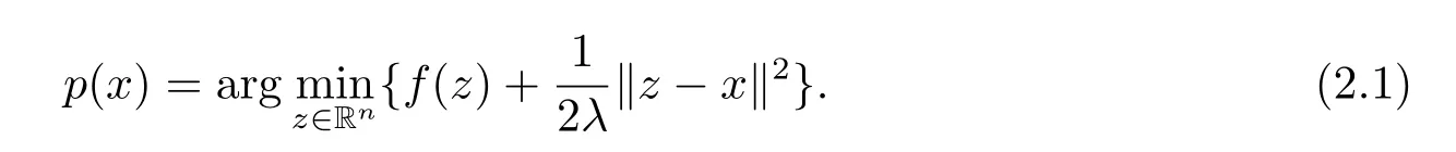
Thenp(x) is the unique minimizer in (1.3).[1]
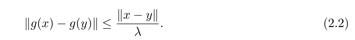
Proposition 2.1The functionFdefined by (1.3) is finite everywhere,convex and differentiable;its gradient isg(x)=∇F(x)=.Furthermore,there holds for allxandyin Rn:
Proposition 2.2The following four statements are equivalent: (i)xminimizesfon Rn;(ii)p(x)=x;(iii)g(x)=0;(iv)xminimizesFon Rn.
Since it is very difficult or even impossible to compute exactly the functionFdefined by(1.3)and its gradientgat a given pointx,we shall use their approximate values.Fortunately,for anyε >0 and a pointx∈Rn,there exists an approximationpα(x,ε) ofp(x) such that

Thus,we can make use ofpα(x,ε) to define the approximations ofF(x) andg(x) by

The above lemma shows that the approximationsFα(x,ε)andgα(x,ε)may be arbitrarily close toF(x) andg(x),respectively,if the parameterεis small enough.
The Perry-Shanno memoryless quasi-Newton-type method for solving the problem (1.2)is described as the iterative formxk+1=xk+akdk,whereak >0 is a step-size obtained by a one-dimensional line search (see next section),anddkis the search direction defined by
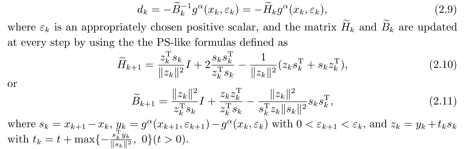
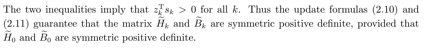
Remark 2.1Note that the formulas (2.10) and (2.11) are obtained by modifying the classical PS method[17].This approach originates from a modification on the BFGS method[20]which guarantees the global convergence without convexity assumption.

3.New Method
In this section,we introduce a modified line search scheme,and then state our PS method for solving the problem (1.2).We also give a remark on the proposed method.

Remark 3.1The MLS (3.1) may be viewed as a modified version of the line search scheme in [21-22].In fact,ifεk →0,the line search scheme (3.1) behaves like the line search scheme in [21-22],due to (2.6).Furthermore,it follows from Lemma 4.1 below that the MLS(3.1) is well defined,i.e.,at thek-th iteration,αkcan be determined finitely.
Now we state our Perry-Shanno memoryless quasi-Newton-type algorithm for solving(1.2) as follows.
Algorithm 3.1
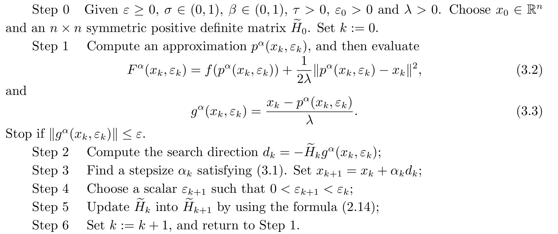
Remark 3.2From Step 1 of Algorithm 3.1,we can see that the calculation ofpα(xk,εk)plays an important role the implementation of Algorithm 3.1.In practice,the approximationpα(xk,εk) can be found by some implementable procedures[1,18]at thek-th iteration.
4.Convergence Analysis
This section is devoted to analyzing the global convergence of Algorithm 3.1.For this purpose,we need the assumption as follows.
Assumption AThe setL0defined as

is bounded,where the initial pointx0is available.
Remark 4.1As suggested in [11],the above assumption is a weaker condition than the strong convexity offas required in [7-8].
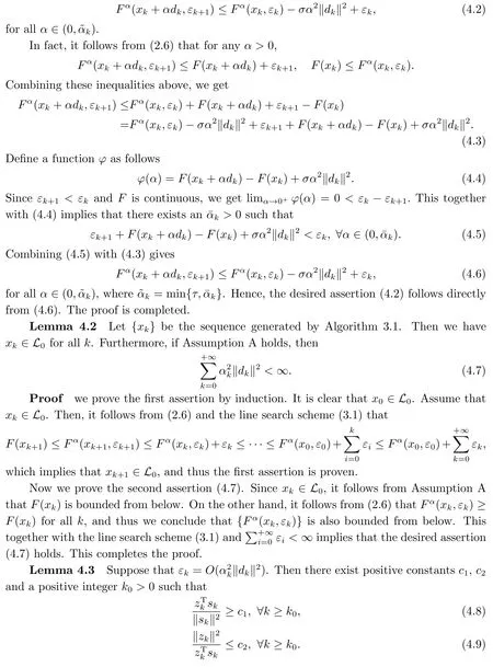
Lemma 4.1Algorithm 3.1 is well defined,i.e.,at thek-th iteration of the algorithm,the stepsizeαkcan be determined finitely in Step 3.
ProofIt suffices to show that at thek-th iteration,there exists an>0 such that


This together with Proposition 2.2 implies thatx*minimizesF.The proof of part two is completed by noting the equivalence of problems (1.1) and (1.2).
Remark 4.3From the convergence analysis in this section,we can see that the value of positive parameterλdoes not affect the global convergence of Algorithm 3.1.However,it can determine the accuracy ofF(x) approximation tof(x) (see [1] for details),thus affecting the convergence speed of our algorithm.Numerical experiments show that choosing an appropriateλmay result in faster convergence than the usual choice (i.e.,λ ≡1) (see[18]).Therefore,although it is proved to be feasible in theory,considering the numerical performance of the proposed algorithm,we still assignλa general positive constant without considering its special case (λ ≡1),in order to ensure that the proposed algorithm has more flexibility and higher efficiency in numerical experiments.
5.Numerical Experiments
Some numerical results are reported in this section to evaluate the performance of Algorithm 3.1 on some standard testing functions,which can be found in [21] and listed in Table 5.1,where the last three columnsn,x0andfopsrepresent the number of variable,initial point and optimal function value,respectively.To show the efficiency of Algorithm 3.1 from a computational point of view,we also give its comparison with some other related methods.

Tab.5.1 Testing functions for experiments
Tab.5.2 Numerical results for related algorithms
The codes used are written in Matlab 7.0 and run on a PC computer equipped with HPdx2810SE Pentium(R) Dual-Core CPU E5300 @ 2.60GHZ 2.00GB.When implementing Algorithm 3.1,the parameters used are set as follows:σ=0.001,β=0.5,λ=100,τ=1,We stop the algorithm when the condition‖gα(xk,εk)‖≤10-6is satisfied.
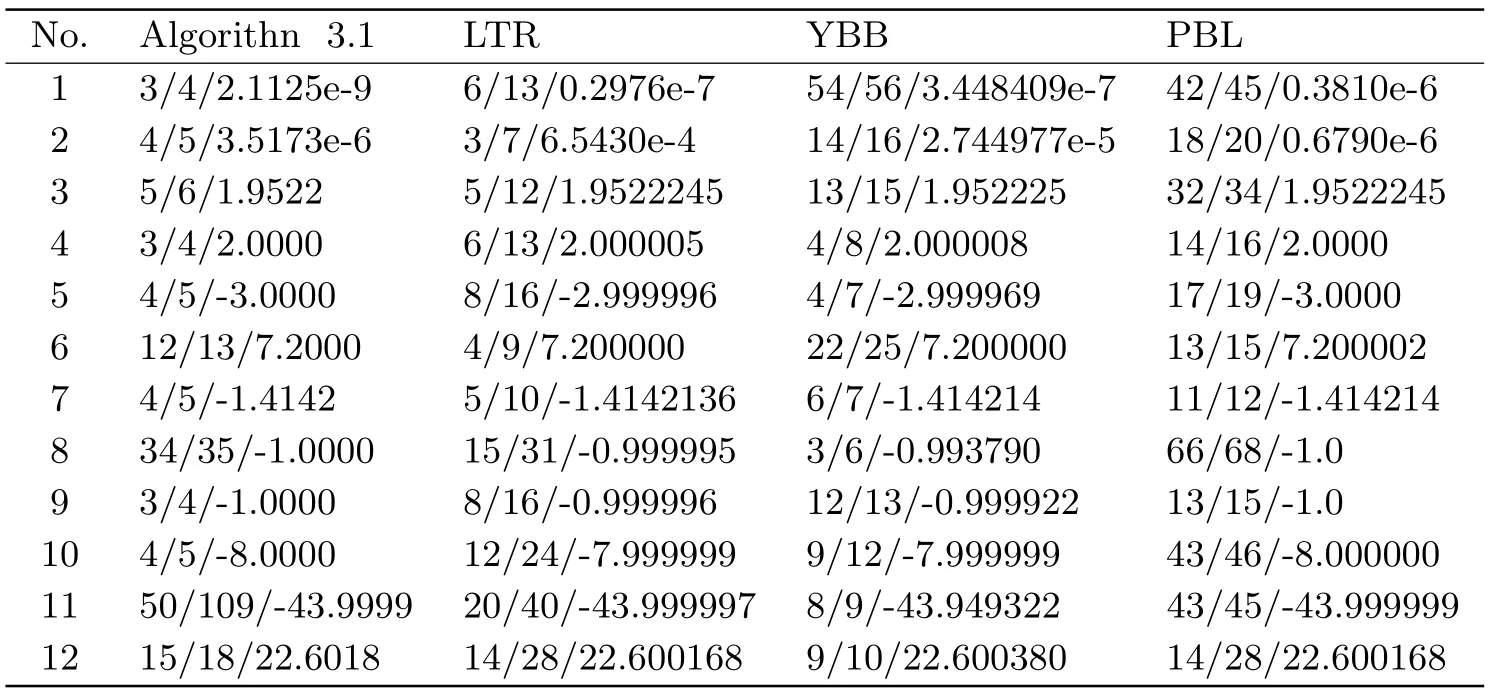
In the first set of numerical experiments,we compare our algorithm with the algorithm in [24] (abbreviated as PBL),the algorithm in [9] (abbreviated as LTR),and the algorithm in [10] (abbreviated as YBB),respectively.The numerical results of these algorithms can be found in [9-10,24],respectively.
Table 5.2 reports the detailed numerical results which are given in the form ofni/nf/fval,whereni,nfandfvalrepresent the number of iterations,the number of function evaluations and the objective function value at termination,respectively.
From the numerical results in Table 5.2,we can find that for most test problems,Algorithm 3.1 performs better than LTR,YBB and PBL in terms of the number of iterations and function evaluations.However,the final function values of the latter are more approximate to the optimal function values than that of the former.
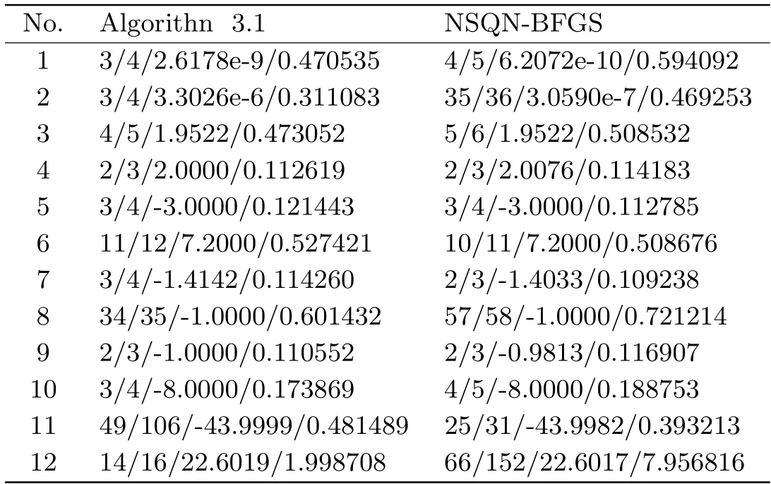
In the second set of numerical experiments,we compare the performance of Algorithm 3.1 with the well-established quasi-Newton method[7](abbreviated as NSQN-BFGS) for the same type of problem and using the same kind of approximation to the function and gradient.Throughout the computational experiments,the related parameters used in NSQN-BFGS are set as follows:ρ=0.5,σ=0.001,ε-1=1,B0=I,γ=0.85 andβk=
Tab.5.3 Numerical results for Algorithm 3.1 and NSQN-BFGS
Table 5.3 reports the detailed test results,which are given in the form ofni/nf/fops/t,wheretdenotes the CPU time in second,while other meanings are the same as those in Table 5.2.From the numerical results in Table 5.3,we can see that for these given problems,Algorithm 3.1 is competitive to NSQN-BFGS in terms of the number of iterations,the number of function evaluations and the CPU time.
While it would be unwise to draw any firm conclusions from the limited experiments,they show some promise for the algorithm proposed in this paper.Further improvement is expected from more sophisticated implementation.
6.Concluding Remarks
In this paper,an implementable Perry-Shanno memoryless quasi-Newton-type method for solving the nonsmooth optimization problem (1.1) has been proposed.It can be viewed as a combination of the Moreau-Yosida regularization with a modified line search scheme and the Perry-Shanno memoryless quasi-Newton method.A feature of the proposed method is that we take advantage of approximate function and gradient values of the Moreau-Yosida regularization instead of the corresponding exact values.Under some reasonable assumption,it is proven that the proposed method is globally convergent.Preliminary numerical results show that the proposed method is efficient to some extent.
It should be emphasized that the proposed algorithm involves finding a vectorpα(x,ε)satisfying (2.3) for givenεandx.Although there are some algorithms that can be used as a procedure to obtain such a vector,it tends to need more iterations whenεis small.Hence,it is interesting to explore some more efficient methods of findingpα(x,ε) to improve the efficiency of the proposed algorithms in the future study.
In addition,the positive parameterλmay affect the performance of the algorithm,Therefore,how to effectively choose this parameter to obtain better efficiency is also our future work.

- 应用数学的其它文章
- 一类线性离散时间系统的预见控制器设计
- Global Boundedness to a Quasilinear Attraction-repulsion with Nonlinear Diffusion
- Trudinger-Moser Inequality Involving the Anisotropic Norm with Logarithmic Weights in Dimension Two
- 关于非齐次树指标m重马氏信源的一个强极限定理
- 相依风险结构下弹性ò休c金产品价Š风险比较
- Superconvergence Analysis of Anisotropic Linear Triangular Finite Element for Multi-term Time Fractional Diffusion Equations with Variable Coefficient