
LARGE TIME BEHAVIOR OF GLOBAL STRONG SOLUTIONS TO A TWO-PHASE MODEL WITH A MAGNETIC FIELD*
2022-11-04 09:06
College of Science,University of Shanghai for Science and Technology,Shanghai 200093,China
E-mail: wwj001373@hotmail.com;chengzhen1995@hotmail.com
Abstract In this paper,the Cauchy problem for a two-phase model with a magnetic field in three dimensions is considered.Based on a new linearized system with respect to (c-c∞,P -P∞,u,H) for constants c∞≥0 and P∞>0,the existence theory of global strong solution is established when the initial data is close to its equilibrium in three dimensions for the small H2 initial data.We improve the existence results obtained by Wen and Zhu in [40] where an additional assumption that the initial perturbations are bounded in L1-norm was needed.The energy method combined with the low-frequency and high-frequency decomposition is used to derive the decay of the solution and hence the global existence.As a by-product,the time decay estimates of the solution and its derivatives in the L2-norm are obtained.
Key words two-phase model;magnetic field;strong solution;global existence;decay rates
1 Introduction
1.1 Background and motivation
In this paper,we are interested in a three-dimensional two-phase system with a magnetic field modelling the motion of the mixture of the fluid and particles.The model is stated as

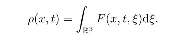
witht≥0 andx=(x1,x2,x3) ∈R3.Here,n,u=(u1,u2,u3) andHdenote the density of the fluid,the velocity field of the fluid and the magnetic field,respectively.ρis the density of the particles in the mixture,which is related to the probability distribution functionF(t,x,ξ) in the macroscopic description through the relation
P=P(ρ,n) is pressure satisfying

forα≥1 andγ≥1.The viscosity coefficientsμandλsatisfy

The constantν >0 is the resistivity coefficient.
In this paper,we will consider the Cauchy problem of (1.1) with the initial data

whereρ∞≥0 andn∞≥0 are two constants.
System (1.1) withα=1 andγ >1 was first formally derived by Wen and Zhu in [40] from the Vlasov-Fokker-Planck/compressible magnetohydrodynamics equations,taking the form of
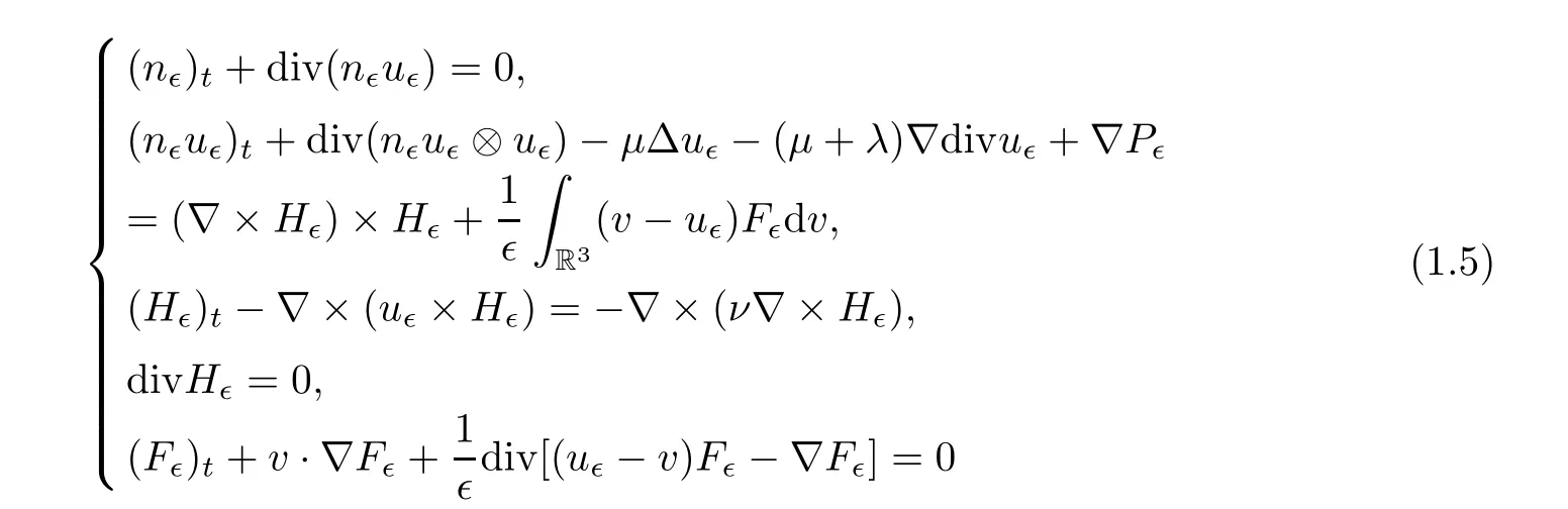
through the scaling limit∈→0+,by applying the ideas of Carrillo and Goudon [3].The system(1.5) describes the motions of the mixture of fluid and particles in magnetic field.This type of fluid-particle interaction system has been widely used in engineering,medicine,geophysics and astrophysics.
There are numerous mathematical results providing insight into the existence,uniqueness and asymptotic behavior of the fluid-particle flows.When omitting the magnetic effect,the global existence of weak solutions to the incompressible Vlasov-Navier-Stokes (without the Fokker-Planck term) system were obtained in [2] by Boudin,Desvillettes,Grandmont and Moussa on a periodic domain and by Yu on a bounded domain in [46].Goudon,He,Moussa and Zhang established the global existence of classical solutions near equilibrium for the incompressible Navier-Stokes-Vlasov-Fokker-Planck system in [17].For the compressible case,Mellet and Vasseur obtained the global existence and asymptotic analysis of weak solutions in[30,31].For when the magnetic effect is involved,there are many studies concerning fluidparticle flows.For the case of fixed∈>0,the first work involving the mathematical analysis of (1.5) was that of Chen,Hu and Wang [5],who investigated the global existence of weak solutions.The gobal existence and large time behavior of classical solutions to the compressible Vlasov-Fokker-Planck/magnetohydrodynamics equations was achieved by Jiang in [22].For the case of the scaling limit as∈→0+,Wen and Zhu [40] established the global well-posedness and decay estimates of strong solutions to system (1.1) when the initial perturbation is small in theH2-norm and itsL1-norm is bounded.Under some smallness assumptions on the intial data but possibly large oscillations,Zhu and Chen,in [49],obtained the global existence of strong solutions as well as the large-time behavior.For more results regarding related fluid-particle models,we refer readers to [4,7,15,27,41,45] and the references therein.
For the general case of (1.2) withα≥1 andγ≥1,the existence of a global weak solution to (1.1) without a magnetic field (where the initial data is large) was established by Vasseur,Wen and Yu [34].They developed an argument of variable reduction for the pressure law which yields the strong convergence of the densities,and provides the existence of global solutions in time for.The caseα,was extended toα,by Wen [37].In [6],Chen and Zhu proved the existence of weak solutions to the steady system of (1.1) without a magnetic field on the condition that the adiabatic constant isα,γ >1 and,γ=1.Coming back to system (1.1),the inviscid case was studied by Ruan and Trakhinin in [33],where a condition sufficient for the local-in-time existence of current-vortex sheets was established.The authors in[33] also achieved the conclusion that contact discontinuities exist locally in time whenα=γ.
The goal of this work is to establish the global existence and decay rates of strong solutions to system (1.1) withα≥1 andγ≥1 when the initial data is a small perturbation in theH2-norm.It is worth pointing out that system (1.1) without a magnetic field is similar to a model called the gas-liquid two-phase model.The main difference between the two systems is that the pressure term in the gas-liquid two-phase model satisfies

whereb1andb2are linear functions with respect to each variable.In this case,there are many results on the global existence and large time behavior of the solutions,c.f.[9–14,18,19,29,35,36,38,39,42–44,48].In particular,Zhang and Zhu [48] established the global existence and optimal time decay rates of solutions to the gas-liquid two-phase model when theH2-norm of the initial perturbation around a constant state is sufficiently small and itsL1-norm is bounded.In [48],the authors introduced an equivalent system for the variable (,P,u) from the gas-liquid two-phase model and derived some a priori estimates ofin theH2(R3)-norm for some constantsn∞andρ∞.It is easy to derive explicit expressions of the functionsandfrom (1.6) on account of the linear features ofb1andb2.However,this does not work for system (1.1) with the equation of state (1.2) for general constantsα≥1 andγ≥1.Fortunately,the difficulty was resolved by Wen and Zhu [40] with a new linearized system of(1.1) with respect to.When the initial perturbation is small in theH2(R3)-norm and theL1-norm is bounded,the authors,in [40],established the global well-posedness and decay estimates of solutions by doing some new a priori estimates to derive the key uniform upper bounds ofn-n∞and.It should be noted that theL1-norm boundedness condition of initial data plays a key role in establishing the global existence of solutions.With the help of this condition,theL2-norm time decay rateof divuwas obtained to handle the linear terms related to divuin the equations ofnandnγ;see Section 3.4 in [40].
Compared with Wen and Zhu’s work [40],only the condition that the initial perturbation is small in theH2(R3)-norm is needed in this paper.Without theL1-norm boundedness condition,one just gets theL2-rateof the term divu,which is not enough to derive the estimateas stated in [40].To overcome this difficulty,our strategy is to introduce a new system (2.2) for the perturbation (c-c∞,P-P∞,u,H),wherecis a new variable defined by (1.7).In this case,the explicit expressions of the functionsρ=ρ(c,P) andn=n(c,P) are obtained in (1.8).At the same time,linear terms related to divuwill not appear in the new equation (2.2)1ofc-c∞.It is obvious thatc-c∞is non-dissipative and thus has no decay-in-time property.In order to close the a priori assumption (3.1),we find that the key point is to obtain the uniform upper bound ofsee Lemma 3.1 for more details.To get around this,we will derive some strong enough decayin-time estimates of the solution~u.The energy method combined with the low-frequency and high-frequency decomposition is used to obtain the decay of the solution,and hence the global existence.Roughly speaking,there are three major types of a priori estimates obtained in the present paper: theestimates on (P-P∞,u,H),theL∞-norm decay estimates of the low frequency part ∇ul,and the weight energy estimateswiths∈(0,) (see Sections 4 and 5).As a by-product,the time decay estimates of the solutions and their derivatives in theL2-norm are obtained.
1.2 Main results
We first rewrite system (1.1) in a more suitable form.Let

Without loss of generality,we focus in what follows on the case ofγ≥α.The case ofγ <αcan be dealt with in a similar way.By a direct calculation,from (1.2) and (1.7)1,we have that

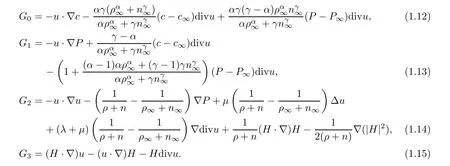
the system (1.1) can be written in terms of the variables (c,P,u,H);that is,
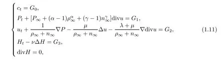
where the source terms are (G0,G1,G2,G3)=(G0,G1,G2,G3)(c,P,u,H) and
The initial data satisfies

We can get the following result for the system (1.11):
Theorem 1.1Assume that (c0-c∞,P0-P∞,u0,H0) ∈H2(R3) for a constantn∞≥0,and thatρ∞≥0,and divH0=0.There is a constantεsuch that if

then the initial data problem (1.11) and (1.16) admits a solution (c,P,u,H) globally in time in the sense that
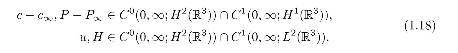
Moreover,there exists a constantsuch that,for anyt≥0,we have the estimates

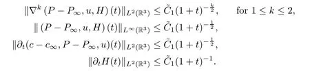
whereK0=‖(P0-P∞,u0,H0)‖H2(R3).Furthermore,for anyt≥0,the solution (c,P,u,H)enjoys the following decay-in-time estimates:
Remark 1.2Whenρ=0,the system (1.1) reduces to the compressible magnetohydrodynamics (MHD) equations.We refer to [20,21,23–25,28,32,47] for the existence theory and the large time behavior of solutions to the compressible MHD equations.
1.3 Notations
Throughout this paper,Cdenotes the generic positive constant depending only on the initial data and the physical coefficients,but which is independent of timet.We will employ the notationa≾bto mean thata≤Cbfor a generic positive constantC.Moreover,the norms in Sobolev spacesHm(R3) andWm,p(R3) are denoted,respectively,by ‖ · ‖Hmand ‖ · ‖Wm,p,form≥0 andp≥1.In particular,form=0,we will simply use ‖·‖L2and ‖·‖Lp.As usual,〈·,·〉 denotes the inner-product inL2(R3).Finally,∇=(∂1,∂2,∂3),∂i=∂xi(i=1,2,3),and for any integerl≥0,∇lfdenotes all derivatives of orderlof the functionf.
The rest of this paper is organized as follows: in the next section,we will reformulate the problem.Section 3 shows some a priori estimates.The decay estimates of the solution are established in Section 4.The proof of Theorem 1.1 is completed in Section 5.In the Appendix,we show some useful inequalities.
2 Reformulations
In this section,to make the calculations as simple as possible,we need to rewrite the system(1.11) by setting
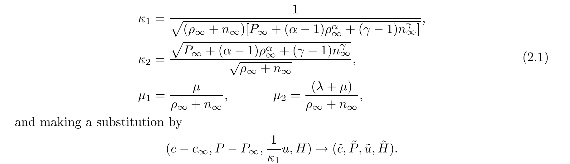
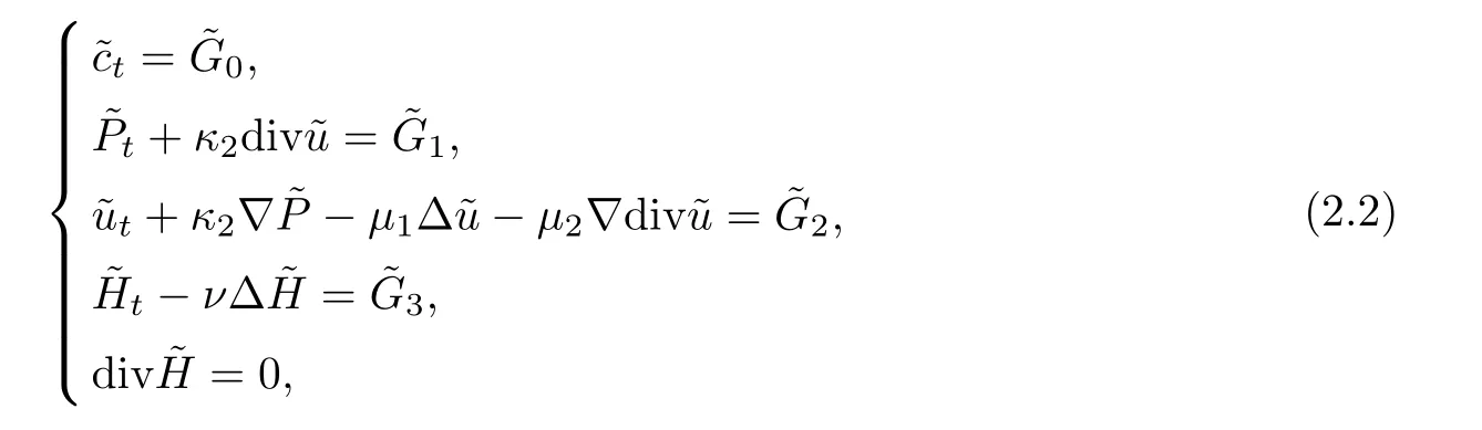
Then system (1.11) becomes

We suppose that the initial data satisfies

In what follows,we will show the existence theory and time decay rates of the solutionto the steady state (0,0,0,0).By a standard continuity argument,the global existence and uniqueness of solutions to (2.2) will be obtained by combining the local existence result with some a priori estimates.

Remark 2.2The proof of Proposition 2.1 can follow the standard argument of the contracting map theorem.We refer to the study of the local existence and uniqueness result in[16] for the compressible MHD system.
Proposition 2.3(a priori estimate) Let∈H2(R3).Assume the initial value problem (2.2) and (2.7) and that there exists a unique global solutionin R3×[0,T] for anyT >0,as well as a constantδ >0 small enough and a positive constantwhich is independent ofT,such that if
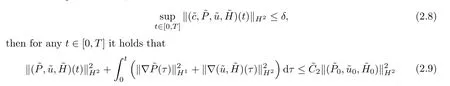
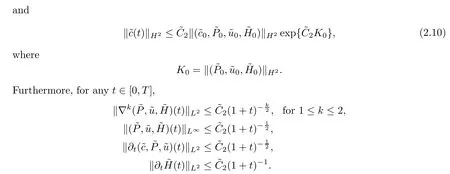
Remark 2.4The global existence and uniqueness of the solution stated in Theorem 1.1 follows from Propositions 2.1 and 2.3.
3 Some A Priori Estimates
In this section,we will show some a priori estimates of the solution.Then,we will establish the decay estimates of the solution.First of all,we make the a priori assumption that
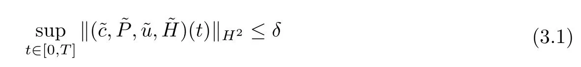
for whenδ >0 is sufficiently small.It follows from (3.1) and the Sobolev inequality that
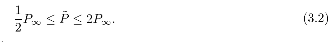
By a direct calculation,one has that

which implies that

3.1 Estimates on (x,t)
In this section,we first show the energy estimate on(x,t).
Lemma 3.1It holds that
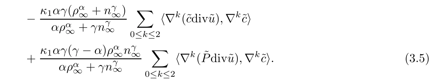
ProofApplying ∇k(0 ≤k≤2) to (2.2)1,multiplying it by ∇k,integrating it over R3,and then summing these up,we have that

For 0 ≤k≤2,by integrating by parts,it holds that

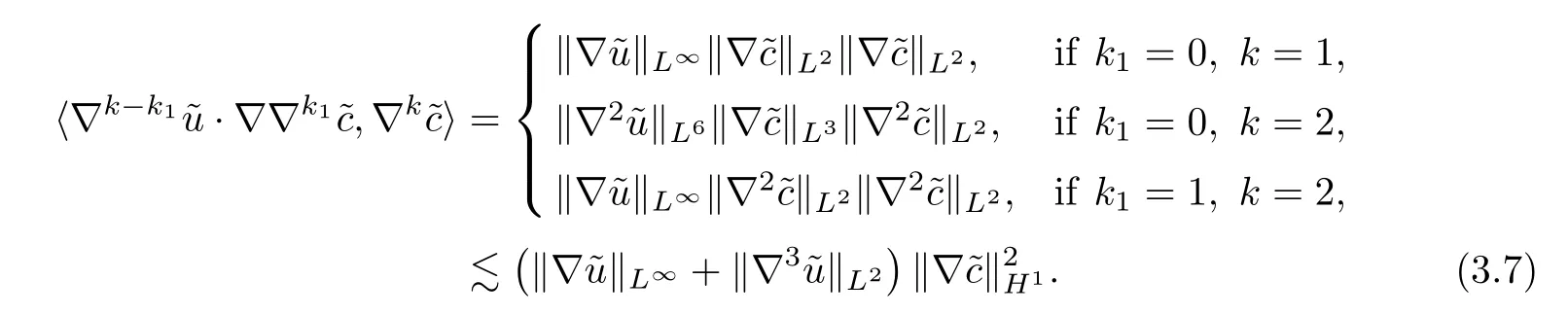
For each 0 ≤k1≤k-1,1 ≤k≤2,by using the Hlder inequality and Lemma A.5,we have that
Similarly,for each 0 ≤k1≤k,0 ≤k≤2,we have that
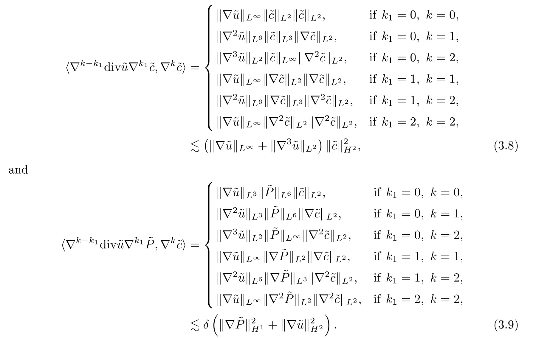
Putting (3.6)–(3.9) into (3.5) yields
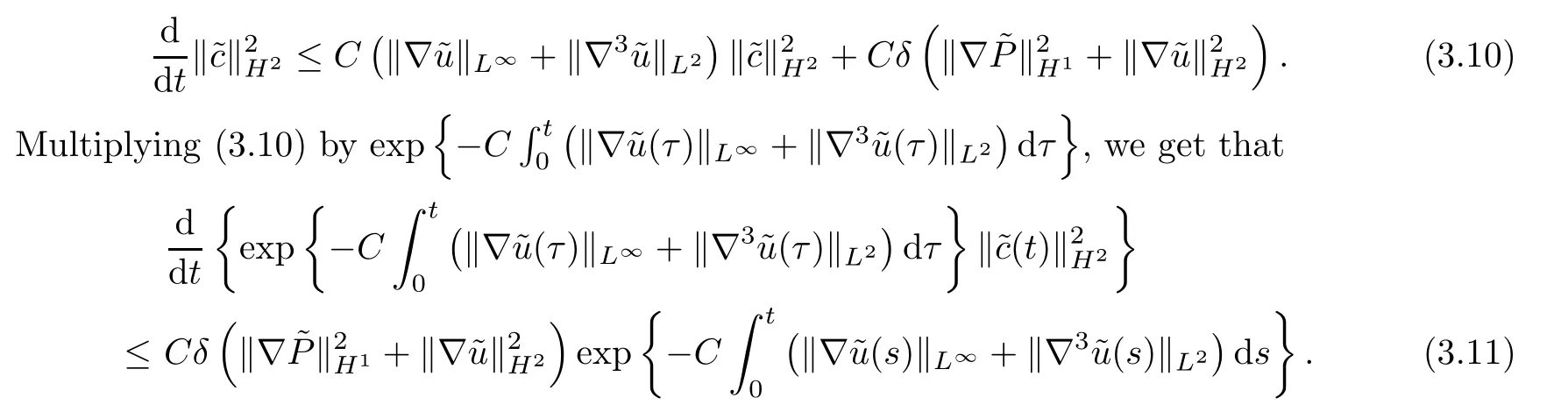
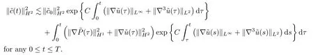
Integrating (3.11) over [0,t],we have that
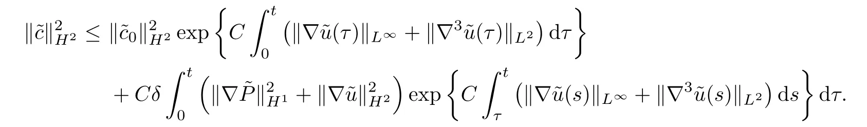
Thus,we have completed the proof of Lemma 3.1. □
3.2 Low-high-frequency decomposition
Based on the Fourier transform,we can define a low-frequency and high-frequency decomposition (fl(x),fh(x)) for a functionf(x) ∈L2(R3) as

whereχ0(Dx) andχ1(Dx),are the pseudo-differential operators with symbolsχ(ξ) and 1 -χ(ξ),respectively.Here,χ(ξ) is a smooth cut-offfunction satisfying 0 ≤χ(ξ) ≤1 and
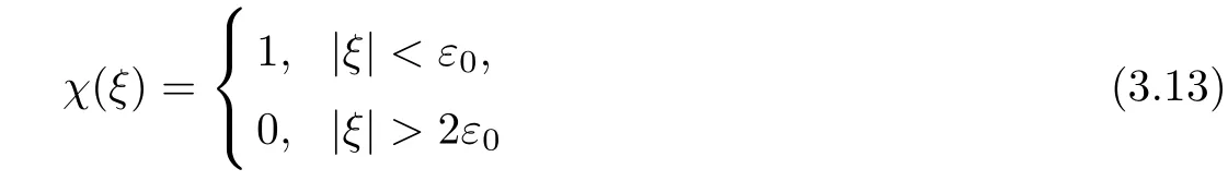
for some fixed constantε0>0.Thus,it is obvious that

Similarly,we can also define a low frequency and high frequency decomposition (fl′(x),fh′(x))forf(x) as


By noticing the definition offh(x) and using the Plancherel theorem,one can get the following lemma:
Lemma 3.2Iff∈H3(R3) is divided into two parts (fl,fh) by the low-frequency and high-frequency decomposition,then there exist two positive constants,,such that

Remark 3.3By noticing the definitions (3.12) and (3.15) and using the Plancherel theorem,one can get that

3.3 Decay estimates of
In this subsection,we will show someLq-norm (2 ≤q≤+∞) decay-in-time estimates of the low-frequency part.Consider the following linearized system related to(2.2):
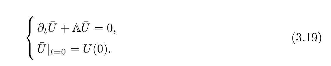

and the solution semigroupE(t)=e-Atis generated by the matrix-valued differential operator A given by

From Theorem 3.1 in [26],one has theLp-Lqtype of the time decay estimates ofEl′(t)=(Dx)E(t) as follows:
Lemma 3.4([26]) Letk≥0 be integers and let 1 ≤p≤2 ≤q≤∞.Then for anyt >0,it holds that

Then the nonlinear system (2.2) can be rewritten as follows:
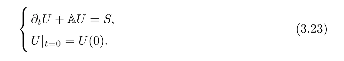
By Duhamel’s principle,we rewrite the solution of (3.23) as follows:
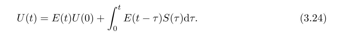
Taking(Dx) on both sides of (3.24),we have that

where we denote the operator.Next,we show the estimates onUl′(t).
Lemma 3.5Under the assumptions of Proposition 2.3,it holds that,for 2 ≤q≤+∞and any integerk≥0,

ProofFrom (3.25) and Lemma 3.4,we obtain that
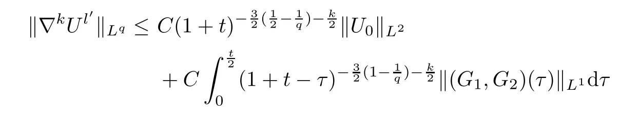
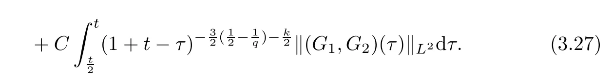
Prior to estimating the 2nd and 3rd terms on the right-hand side of (3.27),we notice that under the conditions (3.1)–(3.4),the nonlinear termsgiven in Section 2 have the following equivalence properties:

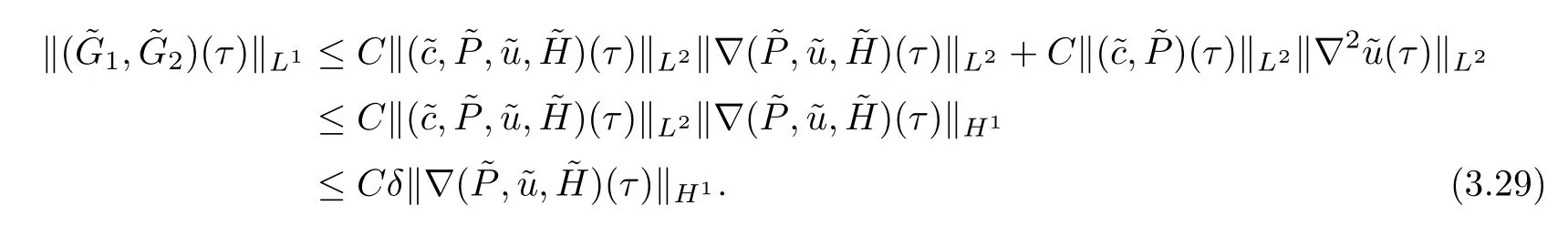
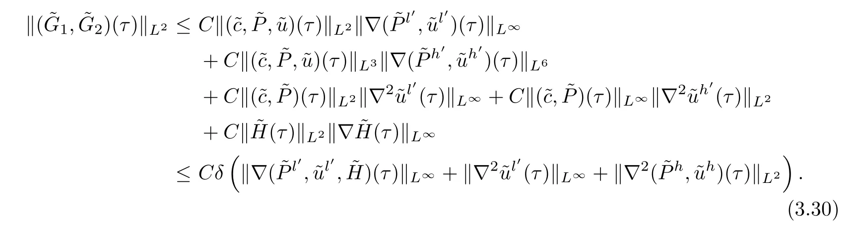
Substituting (3.29)–(3.30) into (3.27),we get (3.26). □
In a similar way,the decay estimates of~Hcan be obtained.The solution of (2.2)4can be written as
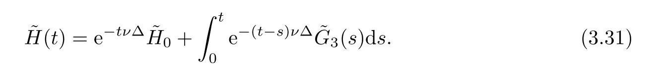
Thus,we have
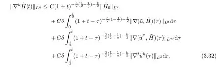
Lemma 3.6Under the assumptions of Proposition 2.3,it holds that,for 2 ≤q≤+∞and any integerk≥0,
3.4 Estimates on
In what follows,we begin to derive the highest order energy estimates on
Lemma 3.7It holds that

for anyt∈[0,T].
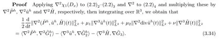
We shall estimate each term on the right hand side of (3.34).The first term on the right hand side of (3.34) can be rewritten as follows:
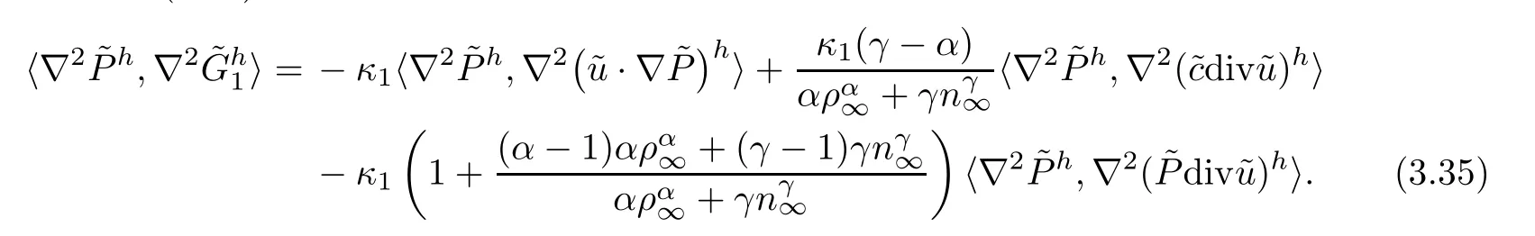
By a direct calculation,we get that
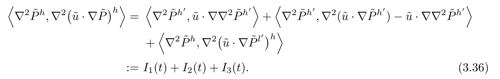
By using integration by parts,Lemmas A.4–A.5,(3.18),the Plancherel theorem,the assumption(3.1) and Young’s inequality,we obtain that

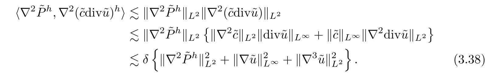
Similarly,we have that

With the above three inequalities in hand,we obtain that

By virtue of the Assumption (3.1),Lemma A.5 and Young’s inequality,we have that
A similar argument shows that

Putting (3.37)-(3.39) into (3.35) yields that

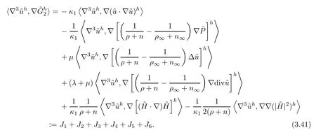
The second term on the right hand side of (3.34) can be rewritten as follows:
Similarly,we get that

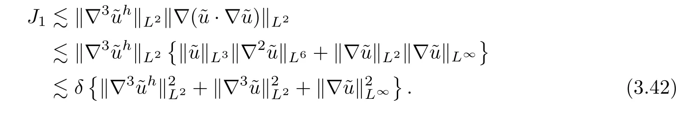
For the term ofJ2,by using the Plancherel theorem,the decomposition (3.16),Lemmas A.4–A.5,(3.4),the Assumption (3.1),(3.18) and Young’s inequality,we have that

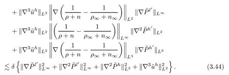
In a manner similar to the proof of (3.44),we get that

Putting the above four inequalities into (3.41) yields that

Similarly to the estimate (3.42),the third term on the right hand side of (3.34) can be estimated as follows:

Substituting (3.40),(3.46) and (3.47) into (3.34) and using (3.16),(3.18) and the smallness ofδ,we get (3.33). □
In the next lemma,we will give the dissipation estimate for(x,t).
Lemma 3.8Under the assumptions of Proposition 2.3,letbe a solution of the initial value problem (2.2) and (2.7).It holds that

for some small constantδ >0.
ProofTaking the operatorχ1(Dx) on both sides of (2.2)3,it is obvious that

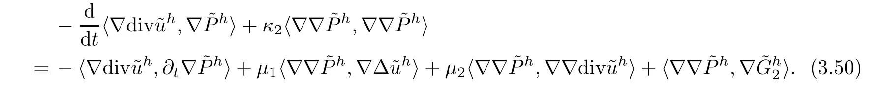
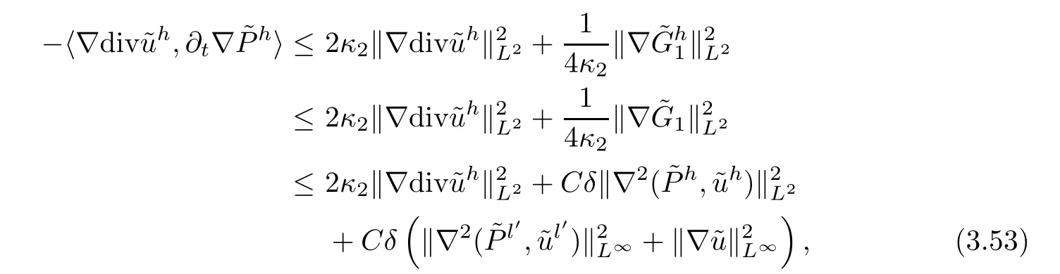
In what follows,we estimate the terms on the r.h.s.of (3.50).By taking the operatorχ1(Dx)on both sides of (2.2)2,we have that

Inserting (3.51) into the first term on the r.h.s.of (3.50),we have that

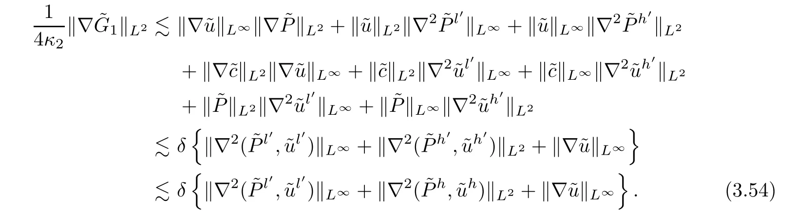
Then,using Young’s inequality,the Plancherel theorem,the decomposition (3.14),Lemma A.5 and the Assumption (3.1),we obtain that
where we have used the fact that
It follows from Young’s inequality and the Plancherel theorem that

For the last term on the r.h.s.of (3.50),similarly to the estimate (3.46),we get that
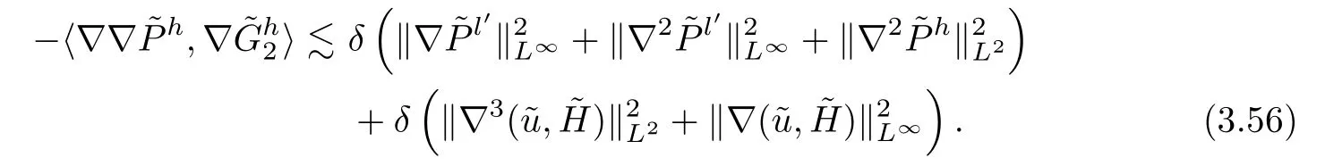
Putting (3.53) and (3.55)–(3.56) into (3.50) and noticing (3.16),(3.18) and the smallness ofδ,we get (3.48). □
As the conclusion of Section 3.1,the following proposition is stated:
Proposition 3.9Under the assumptions of Proposition 2.3,it holds that

where the energy functional H(t) is defined by

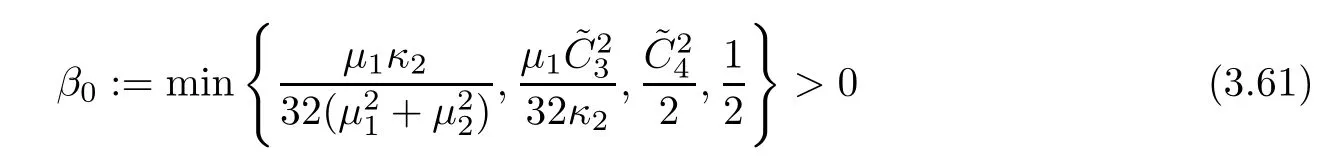
and the positive constant given here,β0,is defined by (3.61).
Remark 3.10It is easy to show that the functional H(t) is equivalent tofor some positive constantβ0;i.e.there exists a positive constantC1independent ofδsuch that

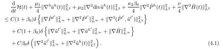
In fact,(3.33)+β0(3.48) gives that

Takingβ0as a fixed positive constant with
and using Lemma 3.2,we have that

Thus,(3.60),together with (3.61),(3.62) and the smallness ofδ,gives (3.57).
According to Young’s inequality and Lemma 3.2,we have that
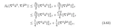
where we have used the fact that,defined by (3.61).Thus,from (3.58) and(3.63),we get (3.59).
4 Decay Rates
In this section,we will establish some estimates of the solutions
Lemma 4.1Under the assumptions of Proposition 2.3,the solutionto the problem (2.2) and (2.7) satisfies that

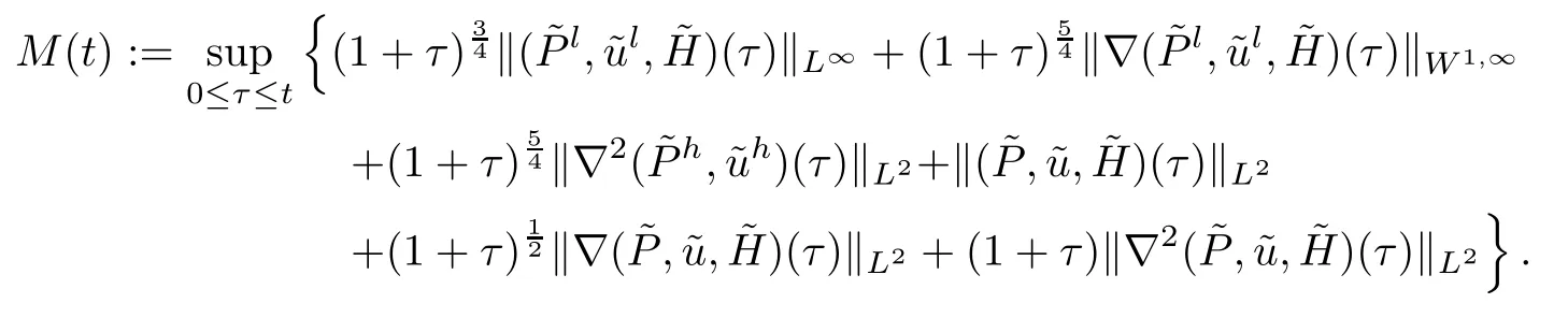
ProofAssume that the solution to the problem exists fort∈[0,T] and denote that
Step 1Due to Proposition 3.9,by the decomposition (3.14),we have that
By virtue of using Lemma 3.2,Lemma A.4,(3.18) and the Plancherel theorem,we have that
By the smallness ofδ,we have that
From (4.4) and (3.59),there exists a positive constantC1such that

Multiplying (4.5) by eC1tand integrating with respect totin [0,t] yields that

Step 2By using Lemma 3.5 withq=+∞and Lemma A.4,fork≥0 we deduce that

It follows from (4.7) and Lemma A.6 that
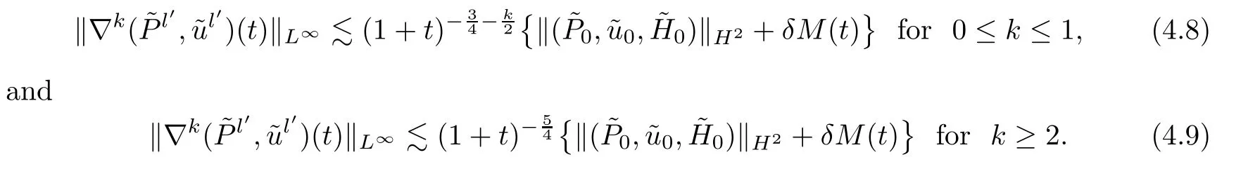
In a similar way,thanks to Lemma 3.5 withq=2,fork≥0 we obtain that
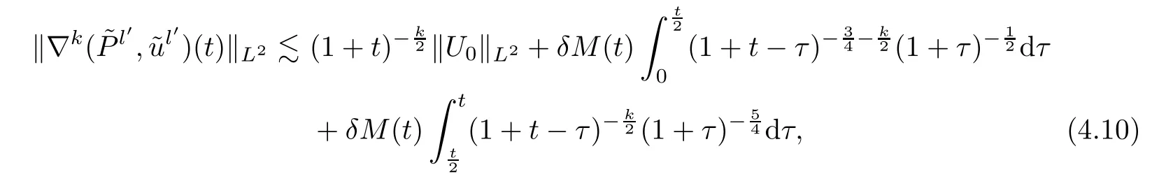
which implies that
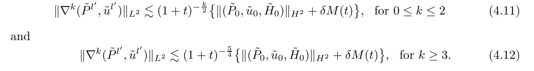
Similarly,we have that

Step 3From (4.6),we get that
It follows from (3.59) and (3.17) that

By virtue of the decomposition (3.16),(3.18),(4.11),(4.15) and (4.17)–(4.18),we have that
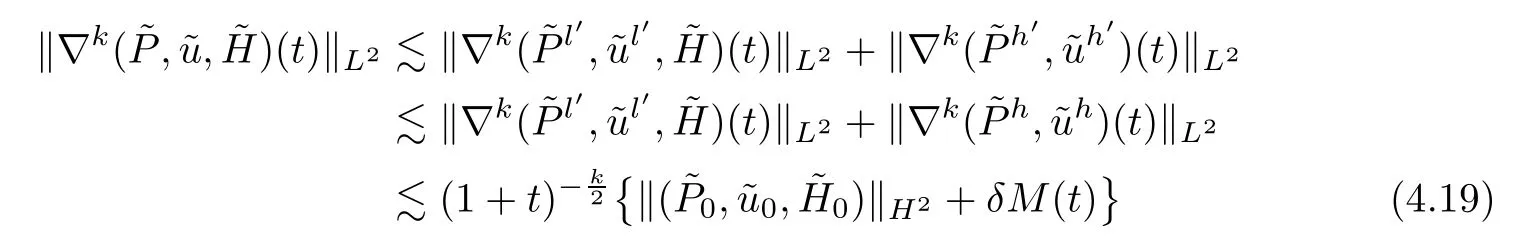
for 0 ≤k≤2.Noticing the definition ofM(t) and using (4.8)–(4.9),(4.11)–(4.16),(4.19) and the smallness ofδ,it is easy to get that

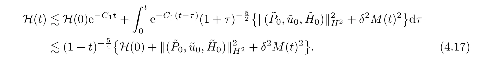
Step 4Multiplying (4.4) by (1 +t)1+swiths∈(0,),we have that
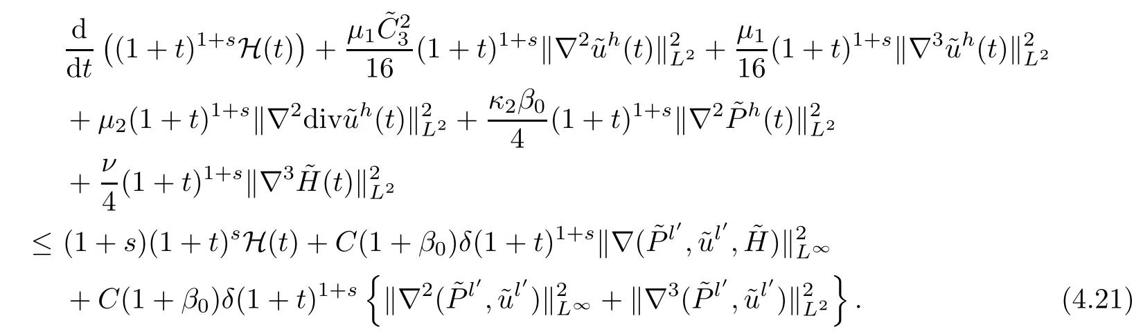
Integrating the above inequality over [0,t] and using (4.8)–(4.9),(4.12),(4.13),(4.17) and (4.20),we get that
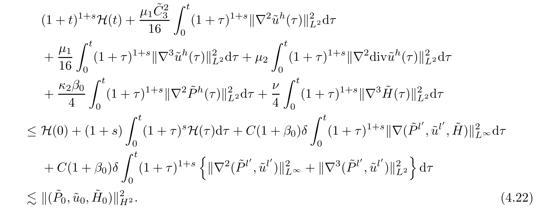
Thus,we have completed the proof of Lemma 4.1. □
5 The Proof of Proposition 2.3
In this section,we first show the energy estimate on (~P,~u,~H)(x,t).
Lemma 5.1It holds that

for any 0 ≤t≤T.
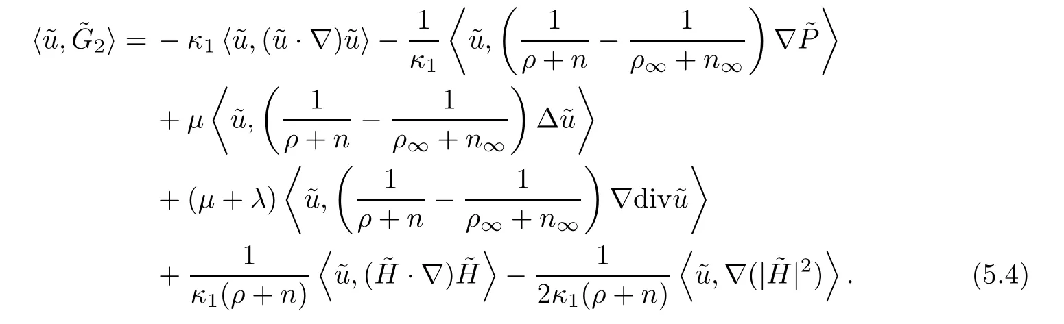
ProofMultiplying (2.2)2,(2.2)3and (2.2)4by,and,respectively,then summing up and integrating the results over R3by parts,we obtain that

The three terms on the right hand side of (5.2) can be estimated as follows: for the first term,using Hlder’s inequality,Lemma A.4,Young’s inequality and the a priori assumption (3.1),we have that
For the second term,we have that
In a fashion similar to the estimate (3.46),it follows from Lemma A.4,Hlder’s inequality and the Assumption (3.1) that

Similarly,we get that
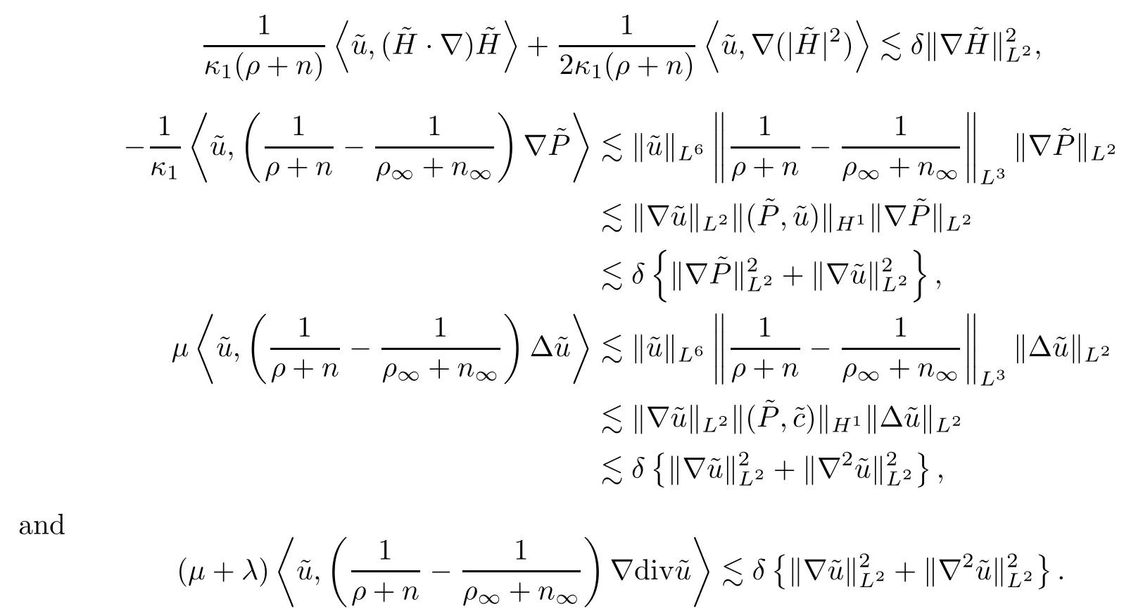
Putting the above five inequalities into (5.4) gives that

In the same way,we have that
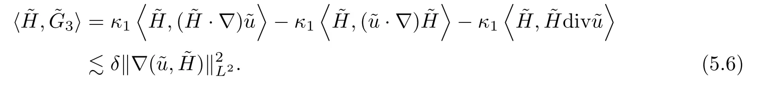
Then,combining (5.3) with (5.5) and (5.6) yields that


sinceδ >0 is sufficiently small.
From (2.2)3,we have that

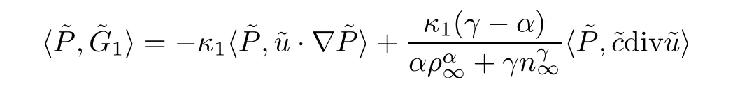
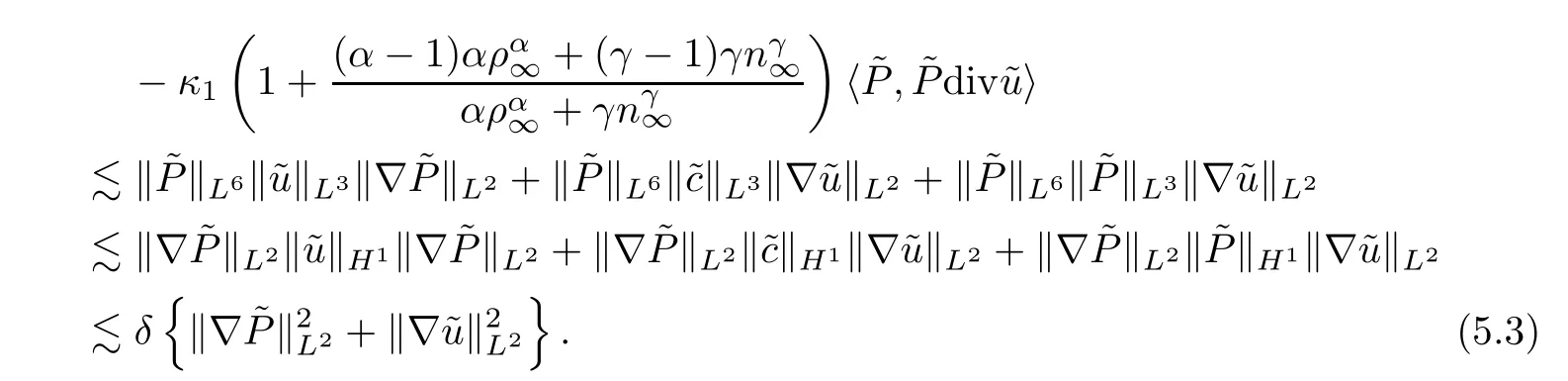
Multiplying this by ∇~Pand integrating the resulting equation over R3,we have that

Using integration by parts and (2.2)2,the first term on the right hand side of (5.9) can be rewritten as
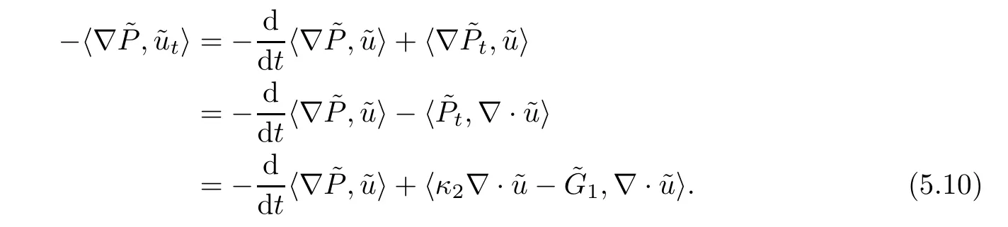
Adding (5.9) and (5.10) and using Young’s inequality,we deduce that


Similarly to the estimate on the term,we have that

Sinceδ >0 is sufficiently small,substituting (5.12) and (5.13) with (5.11) yields that

Finally,multiplying (5.14) byC2suitably small and adding it to (5.7),one has that
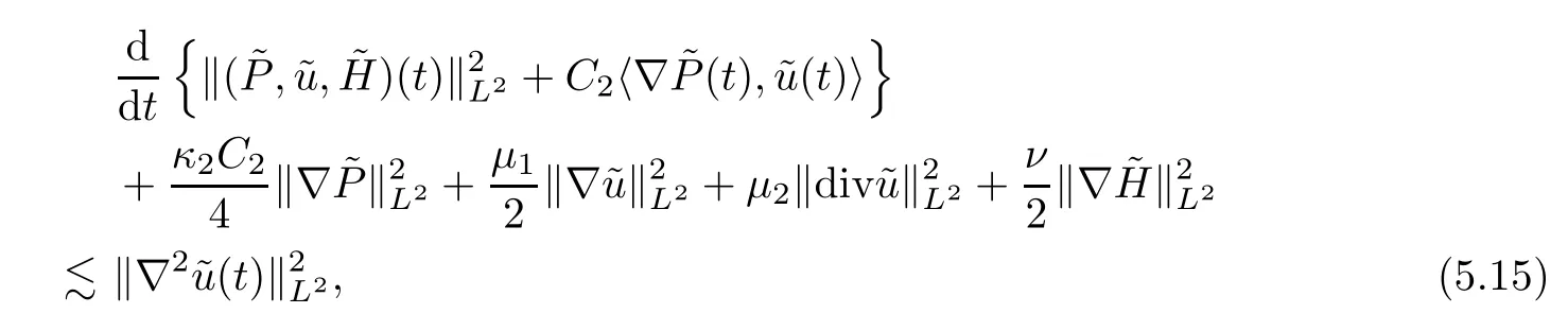
sinceδ >0 is sufficiently small.Integrating (5.15) over [0,t] and using Lemma 4.1 and Young’s inequality,we have that
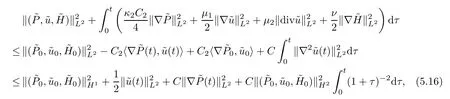
which,with Lemma 4.1,implies (5.1). □
According to Lemma 4.1 and Lemma 5.1,we have
Lemma 5.2It holds that

Now,we will estimate the key uniform upper bound ofwhich,combined with Lemma 5.2,gives the proof of Proposition 2.3.
Lemma 5.3It holds that

for anyt∈[0,T].
ProofIt is obvious that
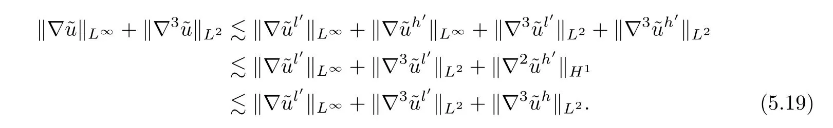
It follows from Lemma 4.1,(4.12) and (4.20) that
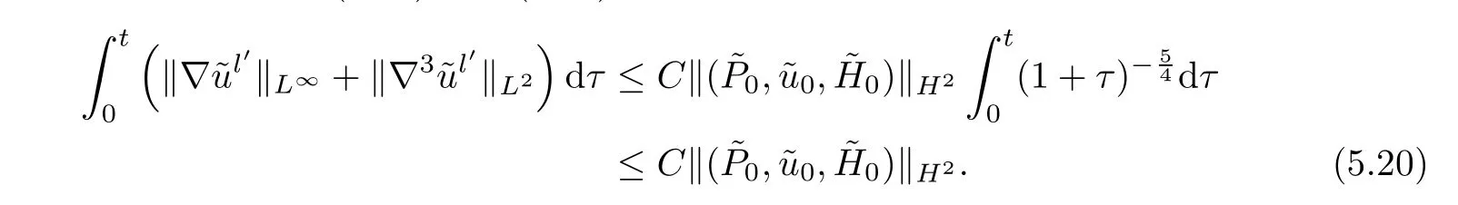
Therefore,we get (5.18). □
By Lemma 5.2 and Lemma 5.3,it follows from Lemma 3.1 that
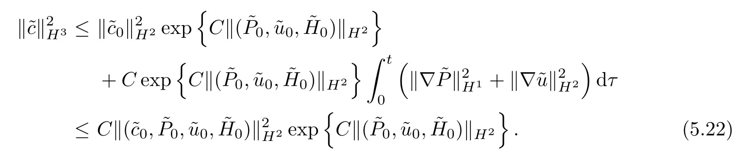
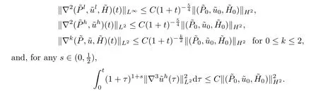
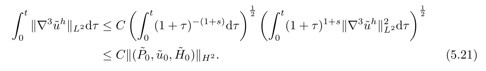
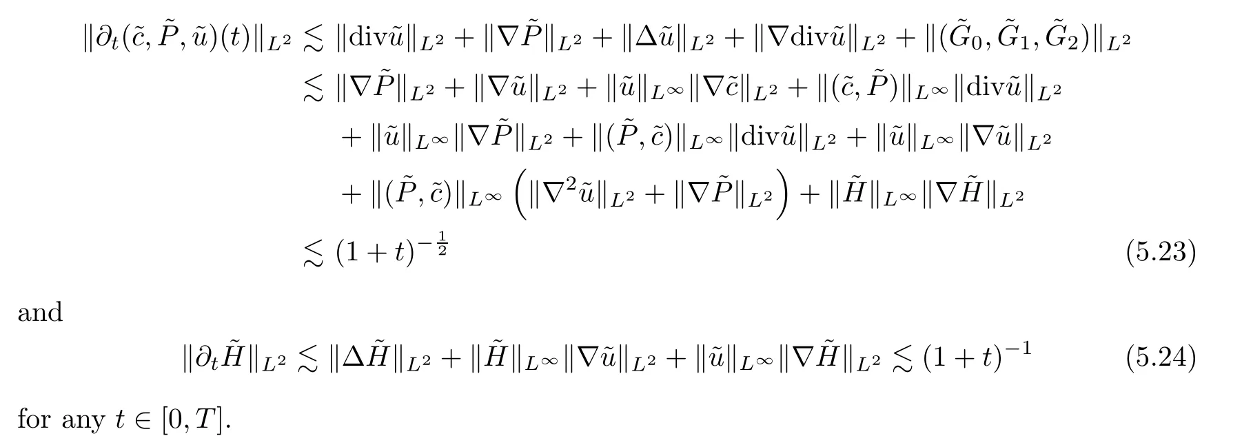
According to Lemma 4.1 and the equations (2.2),we have that
Appendix
In this appendix,we state some useful inequalities in the Sobolev space.The proof of the next lemma can be found in [1].
Lemma A.4Letf∈H2(R3).Then
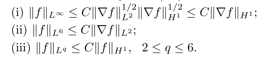
We recall the following lemma (one can find it in [8,35]):
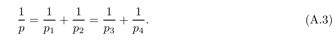
Lemma A.5Lettingm≥1 be an integer,we have that
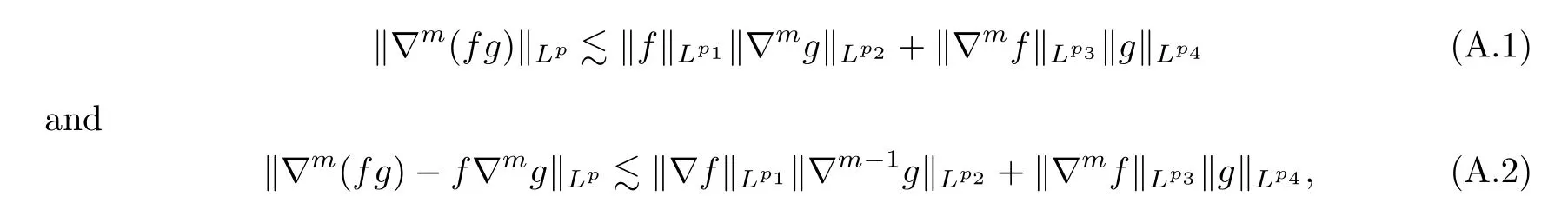
where 1 ≤pi≤+∞,(i=1,···,4) and
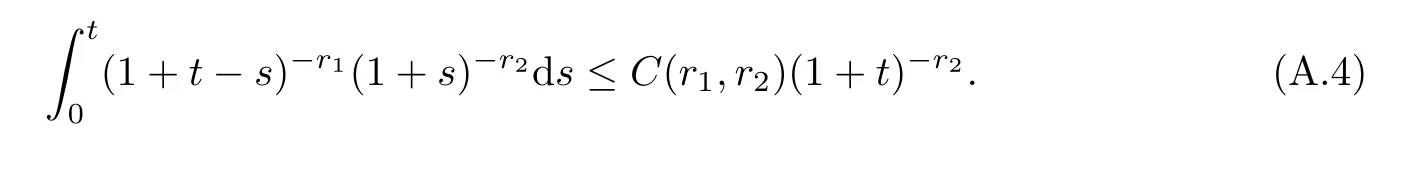
Lemma A.6Ifr1>1 andr2∈[0,r1],then it holds that
 Acta Mathematica Scientia(English Series)2022年5期
- Acta Mathematica Scientia(English Series)的其它文章
- RELAXED INERTIAL METHODS FOR SOLVING SPLIT VARIATIONAL INEQUALITY PROBLEMS WITHOUT PRODUCT SPACE FORMULATION*
- PHASE PORTRAITS OF THE LESLIE-GOWER SYSTEM*
- A GROUND STATE SOLUTION TO THE CHERN-SIMONS-SCHRÖDINGER SYSTEM*
- ITERATIVE METHODS FOR OBTAINING AN INFINITE FAMILY OF STRICT PSEUDO-CONTRACTIONS IN BANACH SPACES*
- A NON-LOCAL DIFFUSION EQUATION FOR NOISE REMOVAL*
- BLOW-UP IN A FRACTIONAL LAPLACIAN MUTUALISTIC MODEL WITH NEUMANN BOUNDARY CONDITIONS*