NUMERICAL ANALYSIS OF A BDF2 MODULAR GRAD-DIV STABILITY METHOD FOR THE STOKES/DARCY EQUATIONS*

College of Mathematics,Taiyuan University of Technology,Tai’yuan 030024,China

E-mail: 996787671@qq.com;menglingxiong@tyut.edu.cn

Xiaofeng JIA (贾晓峰)

School of Mathematics and Statistics,Wuhan University,Wuhan 430072,China

E-mail: jiaoxiaofeng@whu.edu.cn

Hongen JIA (贾宏恩)†

College of Mathematics,Taiyuan University of Technology,Tai’yuan 030024,China

E-mail: jiahongen@aliyun.com

Abstract In this paper,a BDF2 modular grad-div algorithm for the Stokes/Darcy model is constructed.This method not only effectively avoids solver breakdown,but also increases computational efficiency for increasing parameter values.Herein,complete stability and error analysis are provided.Finally,some numerical tests are proposed to justify the theoretical analysis.

Key words Stokes/Darcy model;decoupling method;BDF2 modular grad-div

1 Introduction

In recent years,a lot of attention has been paid to the numerical method for the Stokes/Darcy model,or the Navier-Stokes/Darcy model.So far,many methods have been proposed for solving these models,for example,domain decomposition methods [1],two-grid finite element methods[2],modified two-grid methods [4],characteristic stabilized finite element methods [5],coupled finite element methods [6–8],and so on.An effective tool for improving the quality of the solution for fluid flow in porous media problems is grad-div stabilization [9,10].This technique involves adding 0=-γ∇(∇· u) to the continuous momentum equation;this grad-div term is nonzero and has an effect on the discrete solution.This method was first introduced in[11],and has been widely used in analysis and calculation [12,13].Recently,sparse grad-div stabilization was proposed in [14] to increase the sparsity and to decrease the coupling of coefficient matrices for the velocity created by grad-div stabilization.However,because the matrix stemming from the grad-div term is singular,the larger stabilized parameterγwill cause solver breakdown [15–17].To weaken or avoid this difficulty,modular grad-div stabilization,which is another grad-div scheme with better computational efficiency,was first provided in [18].In [19],a BDF2 modular stabilization method was introduced for the Navier-Stokes equations.In [20],the modular grad-div stabilization method for the time-dependent Stokes/Darcy model was proposed.Meanwhile,many novel extensions of the modular grad-div method were presented in [21–23].In this paper,we come up with a BDF2 modular grad-div stabilization method for the Stokes/Darcy model.This method not only avoids solver breakdown,but also improves the efficiency of the solution and preserve the advantages of the grad-div stabilization method.

The rest of this paper is organized as follows: in Section 2,some notations and the timedependent Stokes/Darcy equation are presented.The BDF2 modular grad-div stabilization method is proposed and the stability analysis is derived in Section 3.In Section 4,under the assumptions of regularity,error estimates for the BDF2 modular grad-div stabilization method are also obtained.In Section 5,compared with the standard scheme,the standard stabilized scheme and the BDF2 modular grad-div scheme,some experiments are presented to verify the theoretical results.The conclusions are presented in Section 6.

2 Functional Setting of the Time-dependent Stokes/Darcy Model

The model we consider is the fluid flow region Ωfcoupled with the porous media flow region Ωp;see Figure 1.Here,Γf=∂Ωf∩∂Ω,Γp=∂Ωp∩∂Ω,and nfand npare the unit outward normal vectors on∂Ωfand∂Ωp,respectively.For the sake of simplicity,we assume that∂Ωfand∂Ωpare sufficiently smooth.

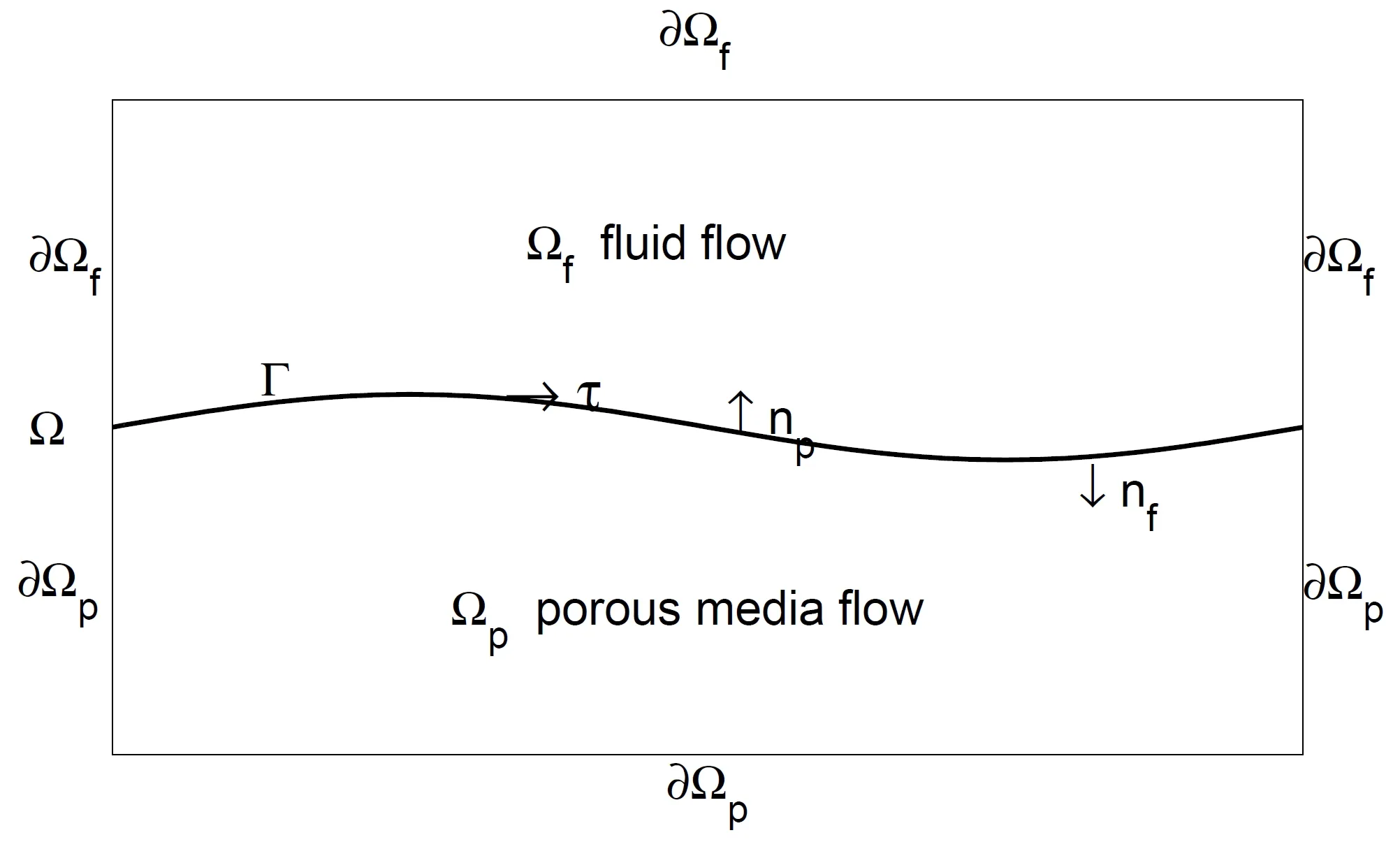
Figure 1 The global domain Ω

The fluid flow in Ωfis governed by the time-dependent Stokes equation

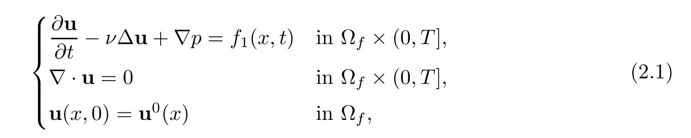
where u=u(x,t) represents the fluid velocity field,p=p(x,t) represents the pressure,the functionf1represents external force,and the coefficientν ＞0 is the kinematic viscosity.

The media flow in Ωpis governed by the Darcy equation

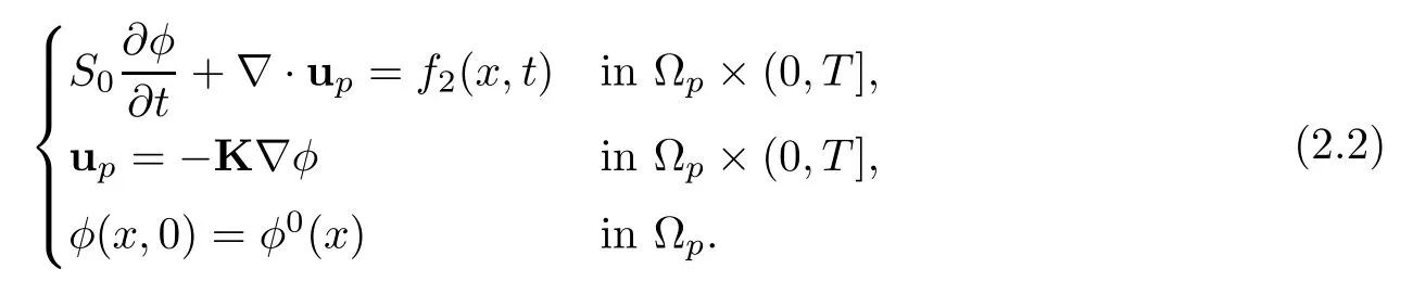
Here,S0is the specific mass storativity coefficient,up=up(x,t) is the velocity,φ=φ(x,t) is the hydraulic head,and functionf2is the source term.K denotes the hydraulic conductivity tensor.For the sake of simplicity,we assume that K is a positive symmetric tensor.

According to Darcy’s law,the second equation in (2.2),the Darcy equation,can be written as follows:

Along with the interface Γ,the interface conditions of the conservation of mass,the balance of forces,and the Beavers-Joseph-Saffman condition are imposed:

Hereτi,i=1,···,d-1 are the orthonormal tangential unit vectors on the interface Γ,gis the gravitational acceleration,andαis a positive parameter depending on the properties of the porous medium and must be determined experimentally.

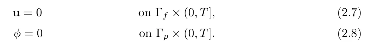
For simplicity,the following boundary conditions on Γf,Γpare imposed:

For the problem (2.1)–(2.8),we introduce the following Hilbert spaces:

The spacesHfandHpare equipped with the following norms:

Here (·,·)Ωdenotes theL2inner product in the domain Ω.Moreover,the discrete norms are defined as follows:

Furthermore,we recall the Poincaré inequality and the trace inequality.There exist positive constantsCpandCtwhich depend only on the domain Ωf,and～Cpand～Ctwhich depend only on the domain Ωp,such that

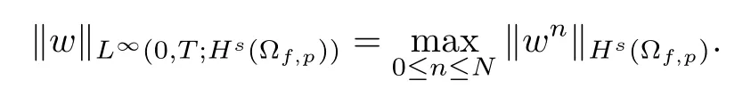
Thus,the weak formulation of the time-dependent Stokes/Darcy model is to findu: [0,T] →Hf,p: [0,T] →Q,φ: [0,T] →Hpsuch that

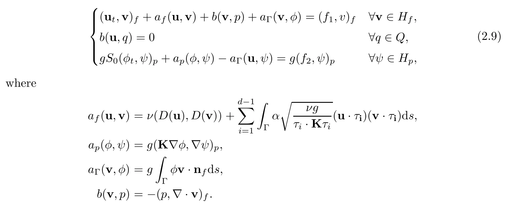
Throughout this paper,Cdenotes the generic positive constant varying in different places but never depending on mesh size,time step or grad-div parameters.The bilinear formsafandapare continuous and coercive:

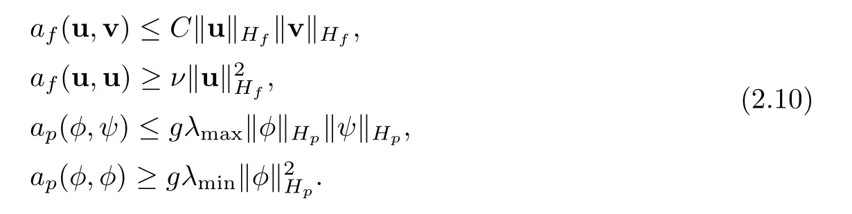
Lemma 2.1([24]) We assume that

HereKis uniformly bounded and positive definite in Ωp,and there exist two constantsλmin＞C ＞0 andλmax＞0 such that

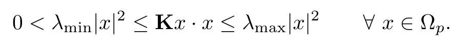
Then any solution (u,p,φ) ∈of (2.1)–(2.8) is also the solution to the equation (2.9).The converse of the statement is also true.

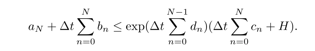
Lemma 2.2([25] discrete Gronwall’s lemma) Let Δt,H,an,bn,cn,dnbe nonnegative mumbers forn≥0 such that,forN≥1,if

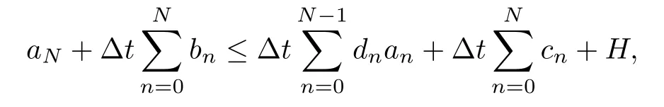
then,for all Δt ＞0,

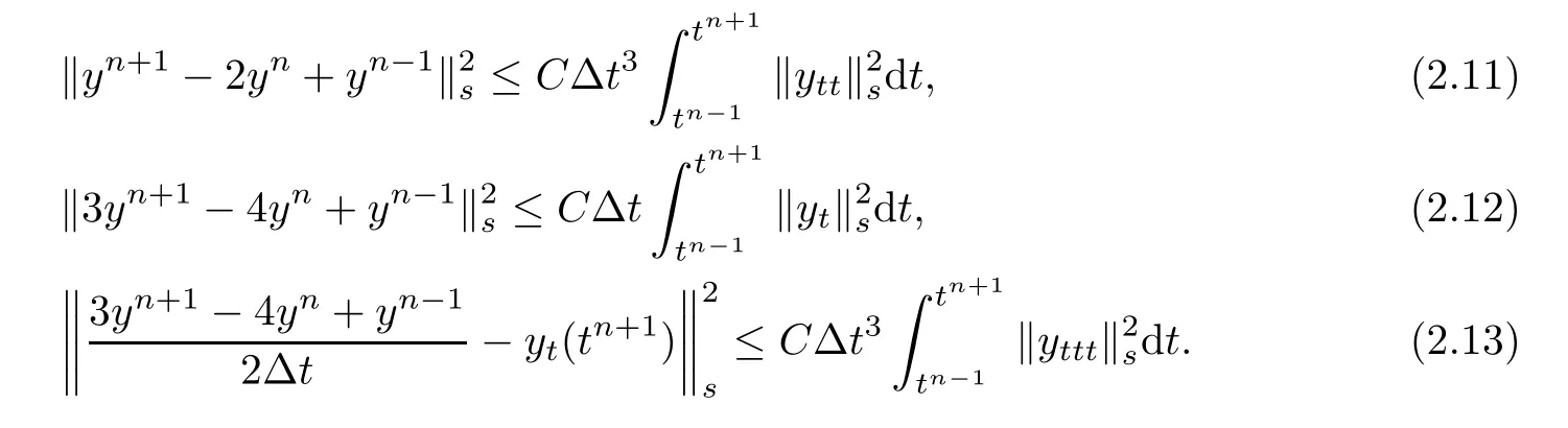
Lemma 2.3([26]) Ifyt,ytt,yttt∈L2(0,T;Hs(Ω)),then we have the following estimates:

3 The BDF2 Modular Grad-div Stabilization Algorithms

We constructτh,which is a quasi-uniform triangulation of the domain Ωf∪Ωp,for any positive parameterh ＞0,which is made up of triangles ifd=2 or tetrahedra ifd=3.Furthermore,we defineHfh,Qh,Hphto be the finite element subspace ofHf,Q,Hp.We assume that the space pairs (Hfh,Qh) satisfy the discrete LBB condition: there existsr ＞0 independent ofhsuch that ∀qh∈Qh,∃vh∈Hfh,vh≠0,

Next,time interval [0,T] is divided into 0=t0＜t1＜···＜tN=Twith Δt=ti-ti-1.Therefore,tm=mΔt,andT=NΔtis a uniform distribution of discrete time levels.Letbe denoted as the discrete approximation of (uh(tn+1),ph(tn+1),φh(tn+1)).

Furthermore,we introduce the inverse inequalities in bothHfhandHph.There exist constantsCIand～CIwhich depend on the domain Ωfand Ωp,respectively,such that ∀vh∈Hfh,∀ψh∈Hph,

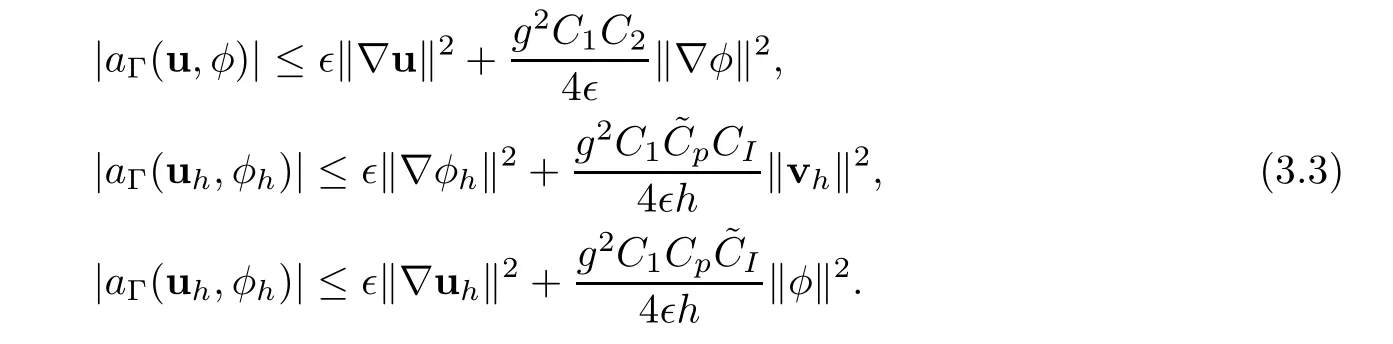
Furthermore,if the finite element spaces satisfy the inverse equality (3.2),the interface coupling termaΓsatisfies the following estimates [27]: there existandC2=such that∈＞0,

We also introduce the discrete divergence-free spaceVh,which is defined as

The BDF2 modular grad-div scheme that was propose can be written as follows:

Algorithm 1(the BDF2 modular grad-div stabilization scheme)

For ∀vh∈Hfh,qh∈Qh,andψh∈Hph:

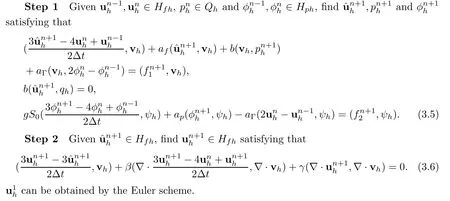
Remark 3.1In this section,conditions are needed for stability.We need for Δtto satisfy that

Next,before analyzing the stability,we introduce a lemma.

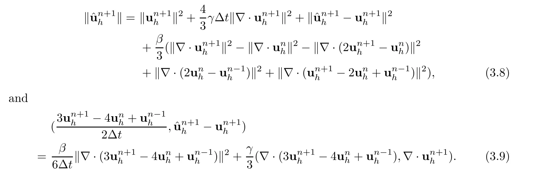
Lemma 3.2For Step 2 (3.6),the following identities hold:

ProofRefer to Lemma 3.2 of [19] for the detailed proof process. □

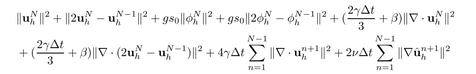
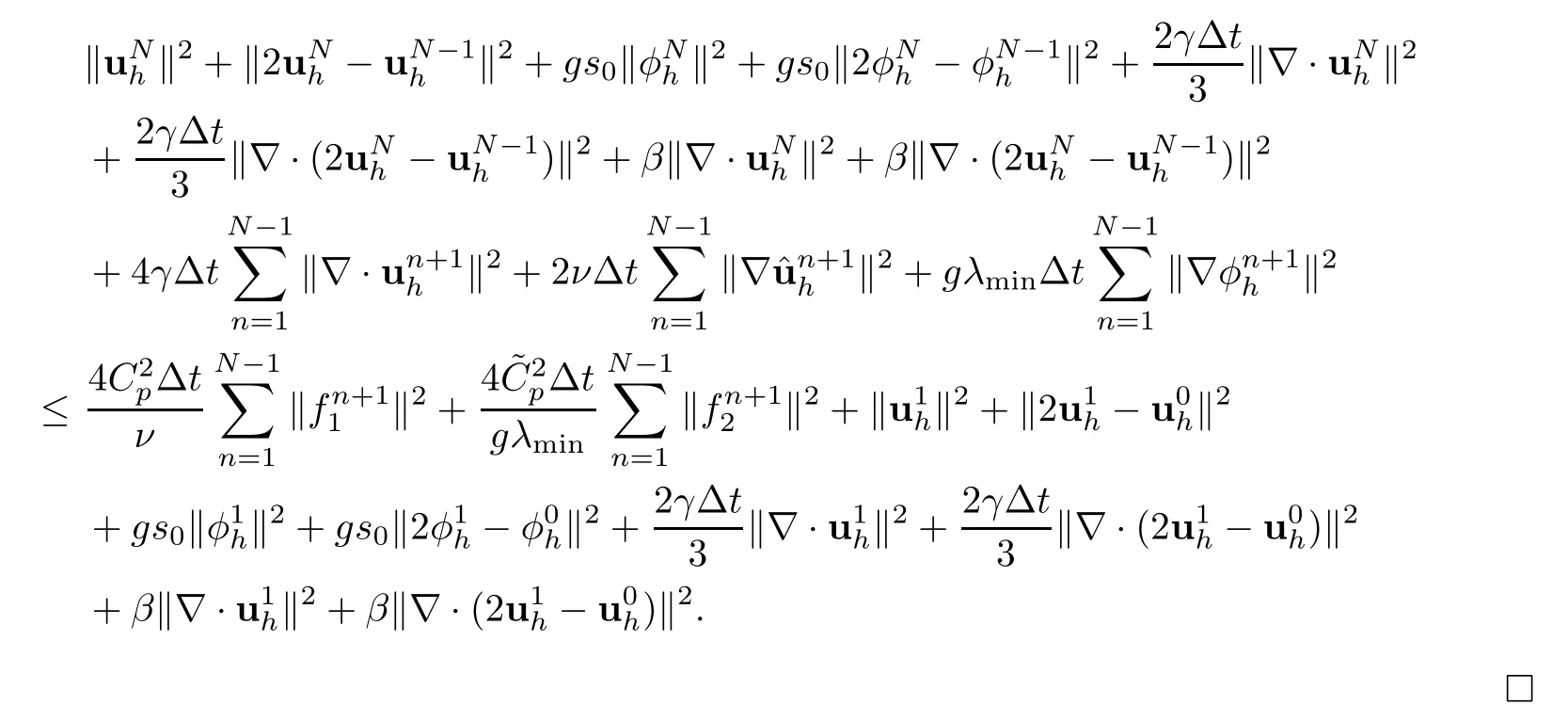
Theorem 3.3(stability) Assume that Δtsatisfies condition (3.7).Then,for anyN ＞1,the solution of the Algorithm 1 (3.5)–(3.6) satisfies that

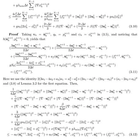
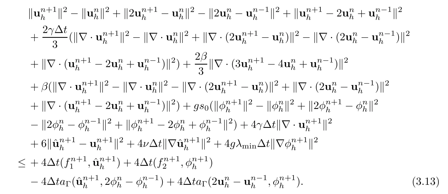
Multiply (3.12) by 4Δtand use (3.9) of Lemma 3.2.This yields that

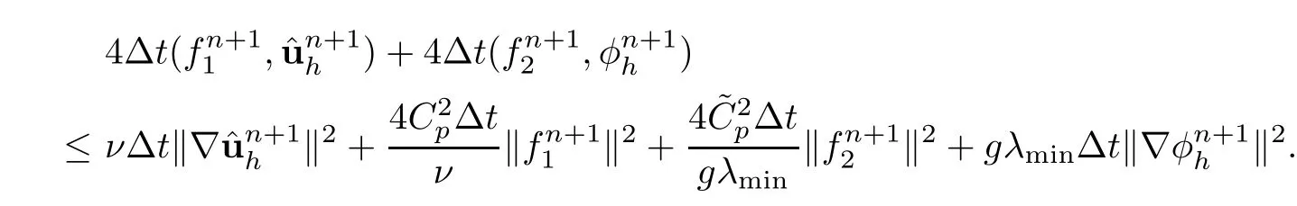
The first term of the right-hand side (RHS) in (3.13) is bounded by the Young-Poincaré-Schwarz inequalities:

The second term of the RHS in (3.13) is bounded by (3.3):

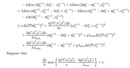
Rearranging the inequality (3.13),using the above inequalities and summing them fromn=1 ton=N-1 and discarding the positive terms on the left-hand side of (3.13),we get the following inequality:

4 Error Analysis

In this section,we will provide error estimates for our proposed BDF2-mgd method.Denote that un=u(tn),pn=p(tn) andφn=φ(tn) forn=0,1,···,N.Assume that the following regularities hold for the true solution:

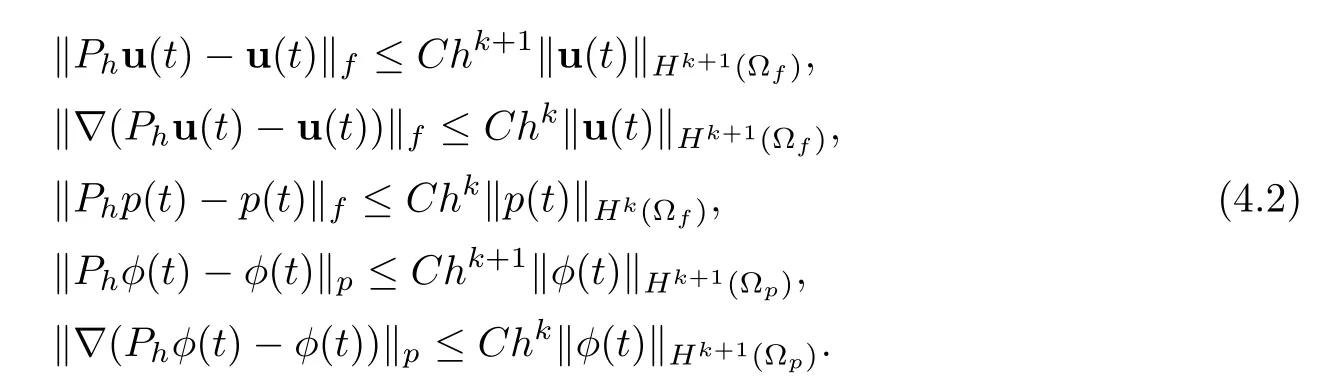
Next,the projection operatorPhcan be defined as [28]

Ph: (u(t),p(t),φ(t)) ∈Hf×Q×Hp→(Phu(t),Php(t),Phφ(t)) ∈Hfh×Qh×Hph.

In addition,(Phu(t),Php(t),Phφ(t)) is an approximation of (u(t),p(t),φ(t)),with the following properties:

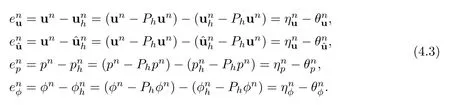
Then,defining the following error equations:

Once again,a crucial lemma is proposed before proving the convergence.

Lemma 4.1For BDF2-mgd (3.5)–(3.6),the following inequality holds:

ProofFor the detailed proof,please refer to Lemma 4.3 in [19]. □

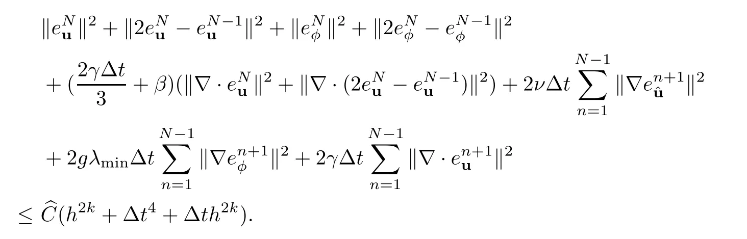
Theorem 4.2Under the regularity assumption (4.1),there exists a constant＞0 independent ofh,Δtsuch that

ProofThe true solution satisfies the following relations:

Subtracting (3.5) and (3.6) from (4.4) and (4.5),we arrive at

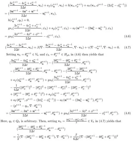
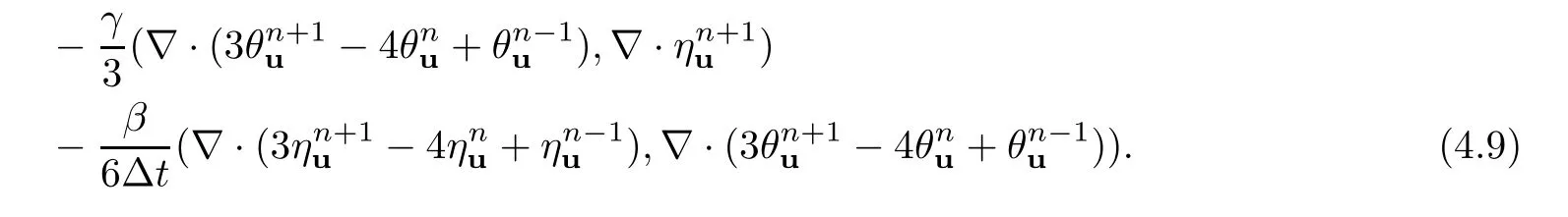
Combining equations (4.8) and (4.9) and rearranging them yields that

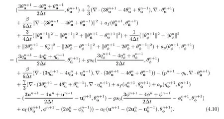
Next,multiplying (4.10) by 4Δtand using Lemma 4.1,we obtain

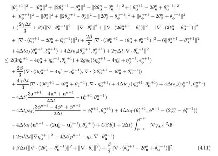
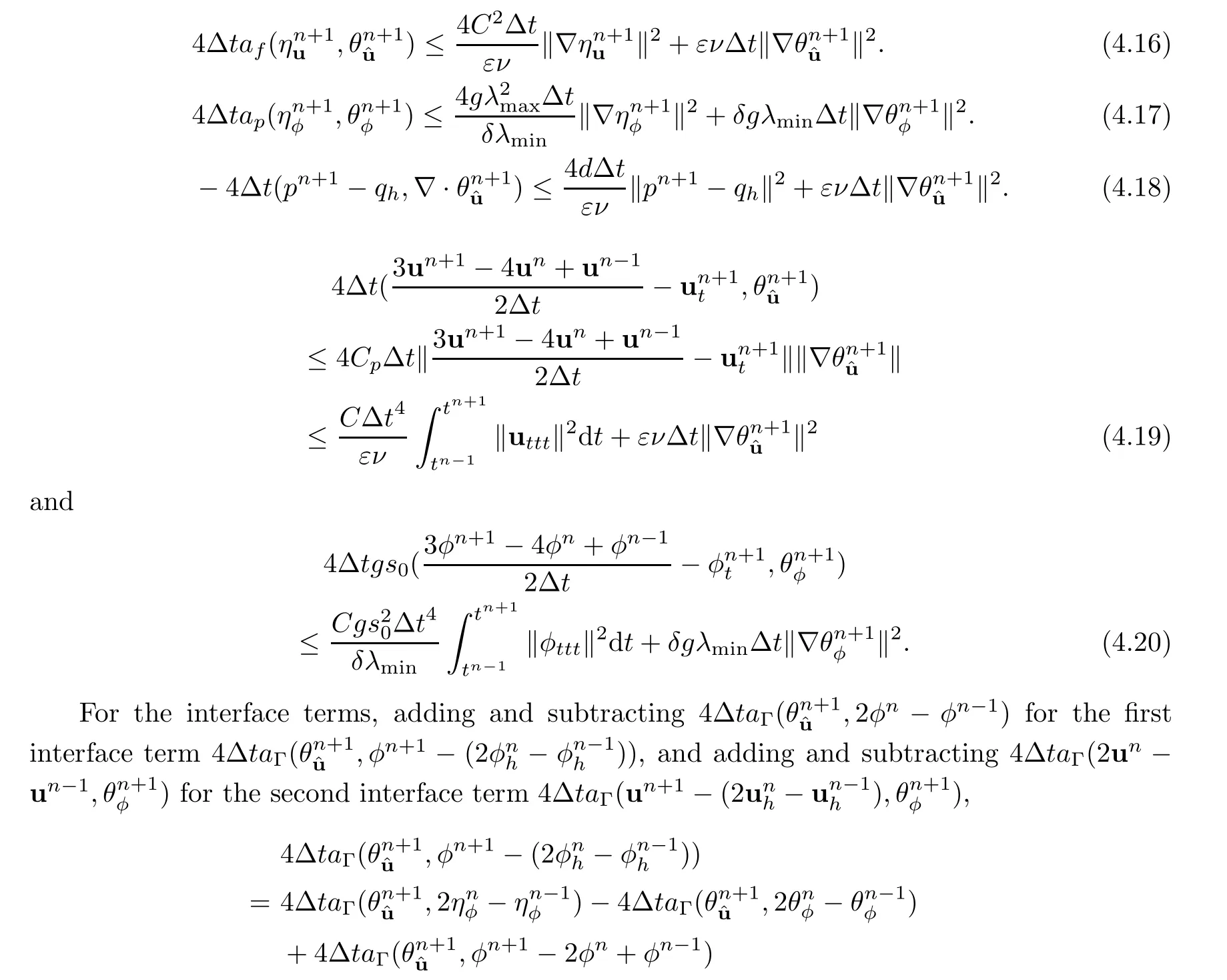
Then,we bound each term on the right hand side of (4.11).Applying Lemma 2.3 and the Cauchy-Schwarz-Young inequality,we have that

Furthermore,

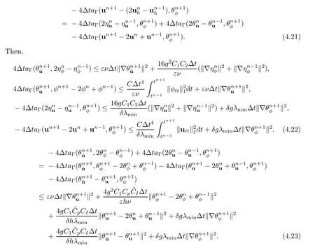
Suppose that

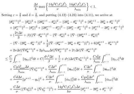
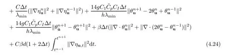
Summing (4.24) fromn=1 toN-1,and discarding the positive terms on the left-hand side of (4.24),we get that

Then,using approximation properties (4.2) and the triangle inequality,the proof is completed.□

Here we can also propose a BDF2 modular grad-div stabilization scheme for the Navier-Stokes/Darcy equations.

Algorithm 2

For ∀vh∈Hfh,qh∈Qh,andψh∈Hph:

5 The Numerical Results

In this section,we compare a standard and stabilized scheme with our BDF2 modular grad-div scheme (3.5)–(3.6).Some numerical tests are performed to confirm the results of the theoretical analysis.The software Freefem++[29] is used in our experiments.

The domain Ω is decomposed into Ωf=(0,1)×(1,2) and Ωp=(0,1)×(0,1) with interface Γ=(0,1)× {1}.The exact solution is given as

In our experiments,the grad-div parameters are selected asγ=1 andβ=0.2,and the physical parametersn,ρ,g,ν,K,S0andαare equal to 1.The initial conditions,the boundary conditions and the forcing terms follow the exact solution.To ensure the accuracy of the results,we set thath=Δt.The famous Taylor-Hood element (P2–P1) and the linear Lagrangian elements (P1) are used for the Stokes problem and the Darcy flow,respectively.The numerical results are presented in Table 1–Table 13.

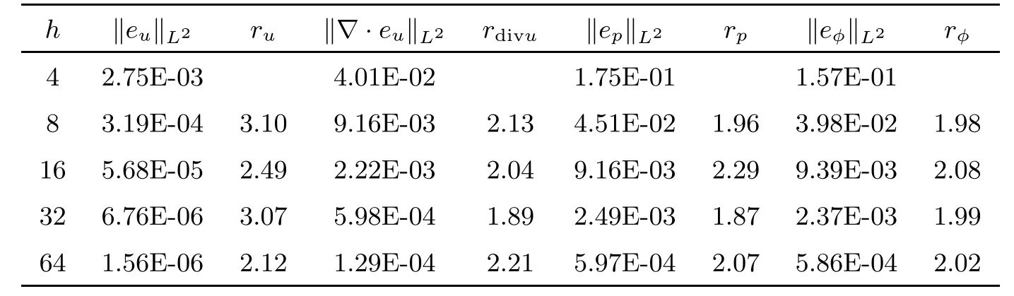
Table 1 Numerical results at time T=1 for the standard scheme with L2 norms

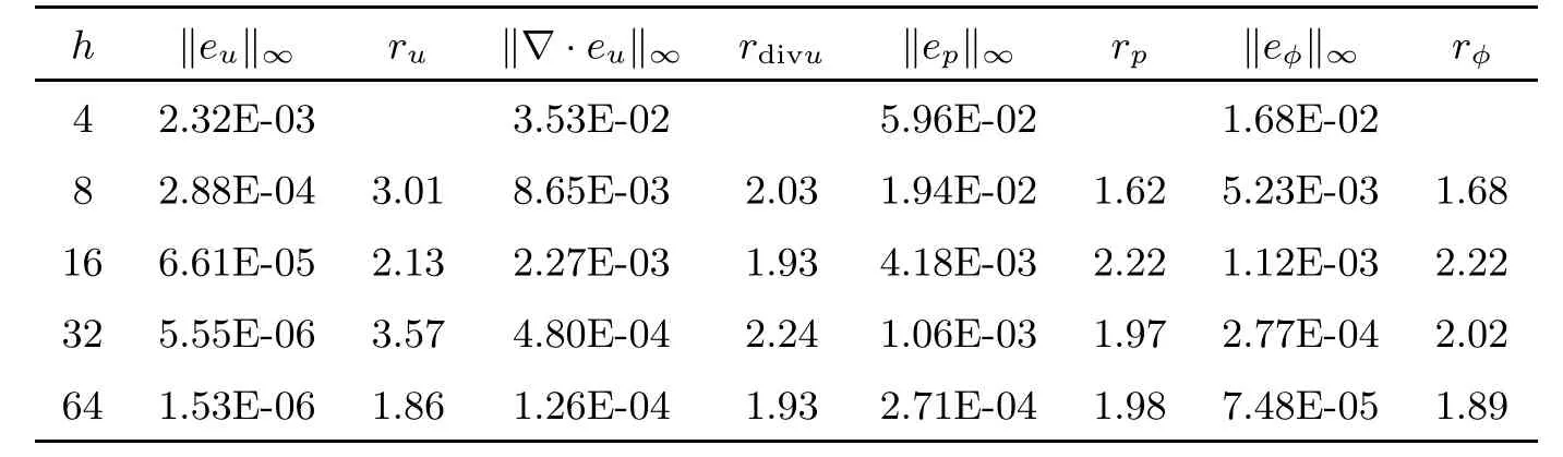
Table 2 Numerical results at time T=1 for the standard scheme with L∞norms

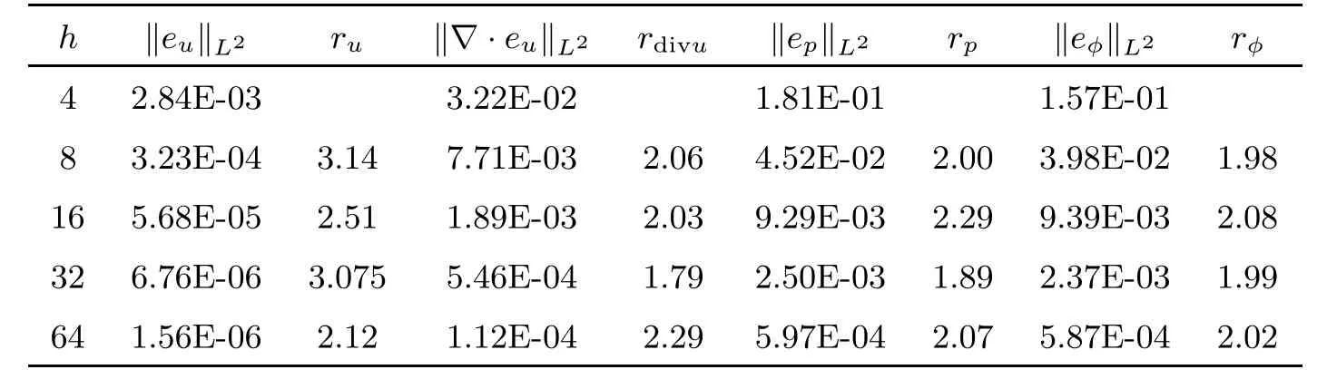
Table 3 Numerical results at time T=1 for the standard stabilized scheme with L2 norms

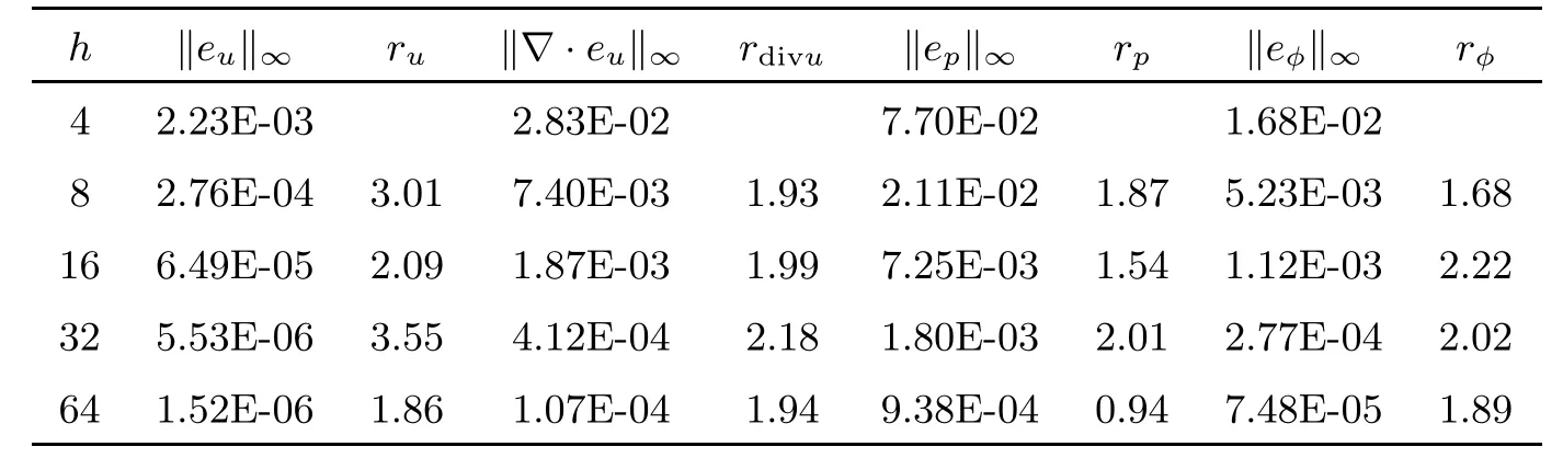
Table 4 Numerical results at time T=1 for the standard stabilized scheme with L∞norms

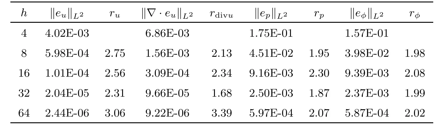
Table 5 Numerical results at time T=1 for the BDF2 modular grad-divscheme with L2 norms

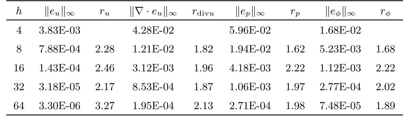
Table 6 Numerical results at time T=1 for the BDF2 modular grad-divscheme with L∞norms

Table 7 Numerical results using P2 for the Darcy component at time T=1 for the BDF2 modular grad-div scheme with L2 norms

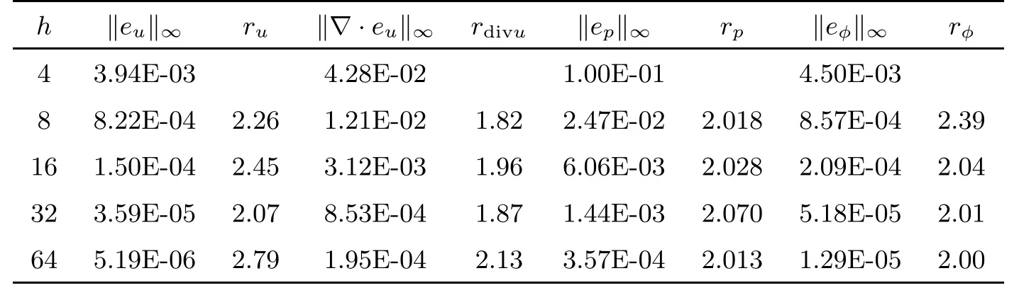
Table 8 Numerical results using P2 for the Darcy component at time T=1 for the BDF2 modular grad-div scheme with L∞norms

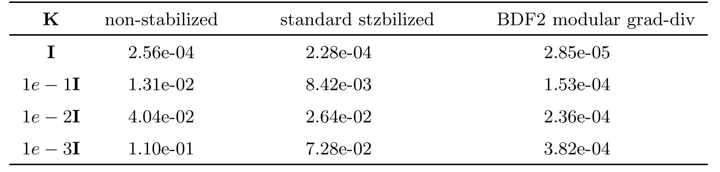
Table 9 The ‖∇· eu‖L2 for the standard scheme,the standard stabilized scheme and the BDF2 modular grad-div scheme with varying hydraulic conductivity tensor K

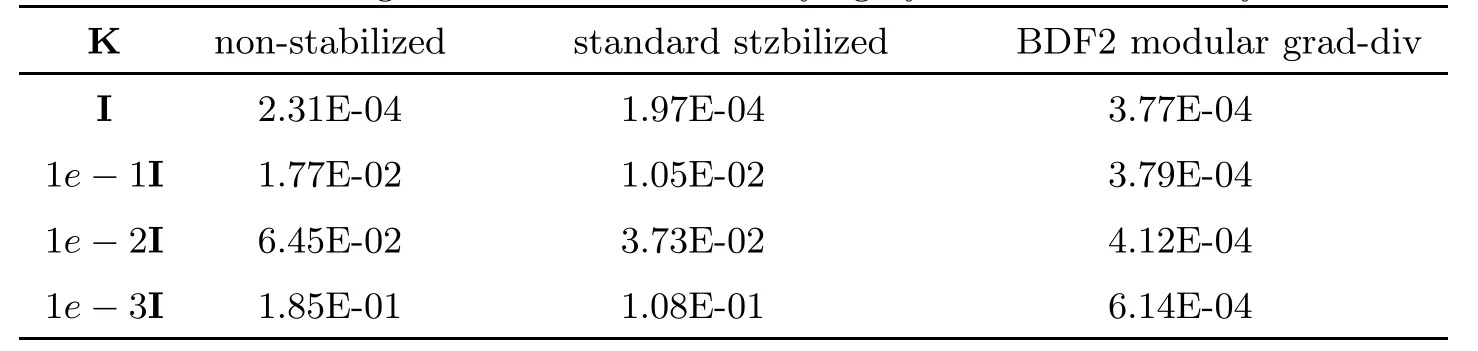
Table 10 The ‖∇· eu‖∞for the standard scheme,the standard stabilized scheme and the BDF2 modular grad-div scheme with varying hydraulic conductivity tensor K

Table 11 The ‖∇· eu‖L2 for the standard scheme,the standard stabilized scheme and the BDF2 modular grad-div scheme with varying hydraulic conductivity tensor ν

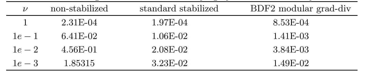
Table 12 The ‖∇· eu‖∞for the standard scheme,the standard stabilized scheme and the BDF2 modular grad-div scheme with varying hydraulic conductivity tensor ν

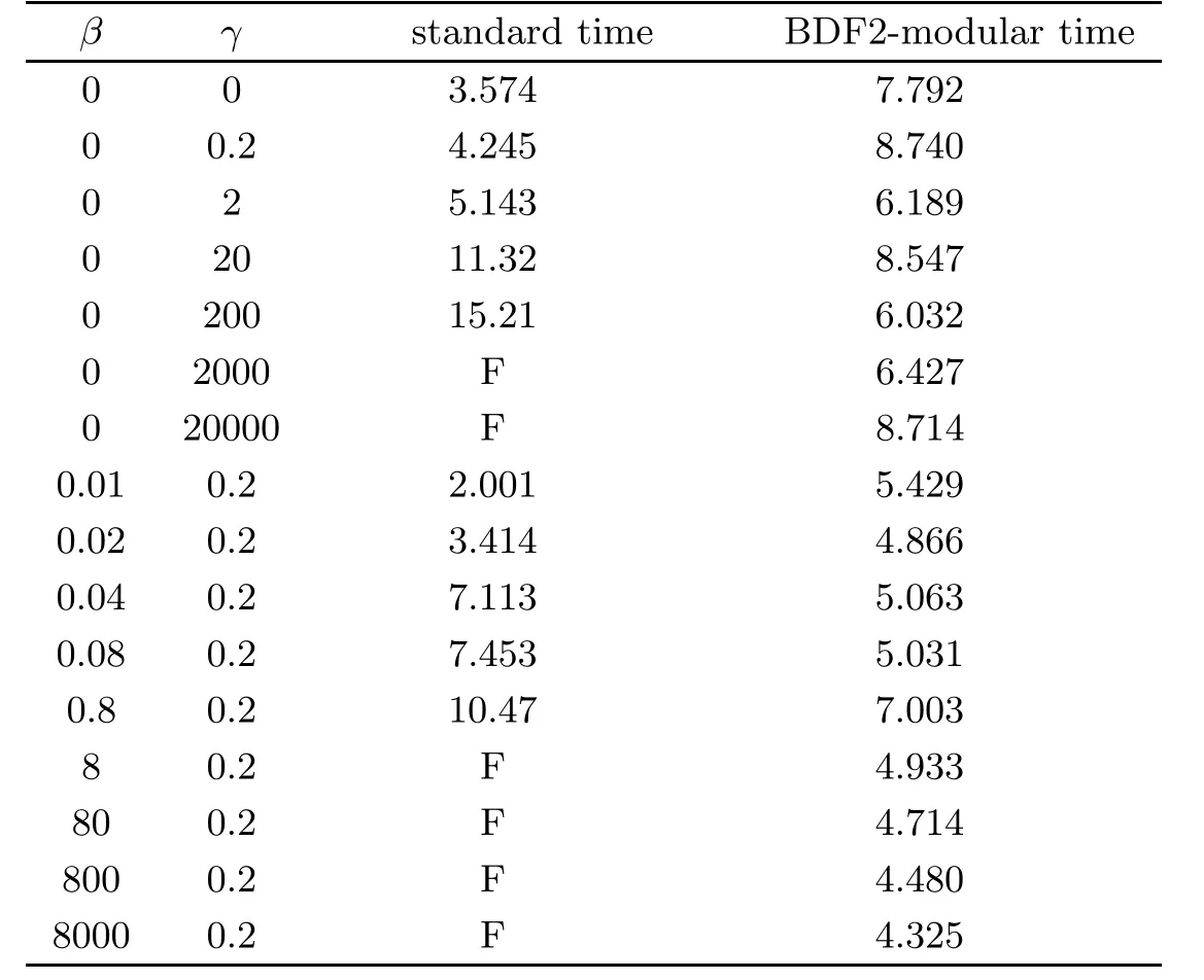
Table 13 Computational time for standard and BDF2 modular grad-div with increasing grad-div parameters

Tables 1 and 2 show the error and convergence order of the velocity u,the pressurepand the hydraulic headφby using the standard scheme.Tables 3 and 4 give the error and convergence order calculated by the standard stabilized scheme.The error and convergence order calculated by the BDF2 modular grad-div scheme are given in Tables 5 and 6.We observe that the divergence velocity errors of the standard stabilized scheme and BDF2 modular graddiv scheme are smaller than those of the standard scheme.In addition,the BDF2 modular grad-div scheme is more accurate.Moreover,the numerical results of both are consisted with the theoretical analysis.To make a comparison using P1 and P2 elements for the Darcy flow,some numerical results are presented in Tables 7 and 8.We observe that the convergence rate for both P1 and P2 elements is close to second-order accurate in time,but the pressure error and the hydraulic head error using the P2 element are smaller than those of the P1 element.

Next,we set up a test to observe the effect of varying K on the errors of the three schemes.We fixν=1 and establish thatTables 9 and 10 show the error of ∇· u for the non-stabilized,standard stabilized and BDF2 modular grad-div schemes with hydraulic conductivity K=I,0.1I,0.01I,0.001I.By observation and comparison,we find that the error for all three schemes increases with a decrease in K.However,the growth is relatively small for the two stabilization schemes.In particular,there is almost no change for the BDF2 modular grad-div scheme.

Then,we consider the issue of pressure-robustness.The grad-div stabilization adds the grad-div parameterγto reduce the lake of pressure-robustness,but does not remove it.Generally,for standard methods,velocity error estimates depend on;it is the same in this paper.However,for standard grad-div methods,pickingγ ＞ν,the scaling of the velocity errorwith the best approximation error of the pressure is reduced fromν-1toν-1/2γ-1/2.Then,we fix K=I,and varyνto investigate the sharpness of our results.The results are presented in Tables 11 and 12.We observe that the velocity errors of the standard scheme grow asνdecreases.For the standard stabilized scheme and the BDF2 modular grad-div scheme,the velocity errors are approximate asνdecreases.This shows that here,the effect ofνis not sharp.

Finally,we compare the computational times of the standard stabilized and the BDF2 modular grad-div stabilized schemes.To test computational efficiency,we fixand varyγandβ.Forγ=β=0,the standard stabilized scheme becomes the standard scheme.For the standard stabilized and the first step of the BDF2 modular grad-div,we use the standard GMRES solver.For the second step of the BDF2 modular grad-div,since it leads to an SPD system with the same sparse matrix,we use the CG solver.If GMRES fails to converge at a single iterate,we denote the result with an “F”.The results are presented in Table 13.Through observation,it can be found that the computational time of the standard stabilized scheme generally increases withγandβ.However,the computational time of the BDF2 modular grad-div scheme is unaffected,and so is increasingly more efficient than the standard stabilized scheme.

6 Conclusion

In this paper,we presented a BDF2 modular grad-div stabilized method for the Stokes/Darcy model.Compared with standard stabilization,our algorithm produces consistent numerical approximations while avoiding solver breakdown for large parameters.We have proven that this scheme is conditionally stable,and error estimates have also been given.Finally,we have performed numerical tests to verify the theoretical analysis and its computational efficiency.