
ST‐SIGMA:Spatio‐temporal semantics and interaction graph aggregation for multi‐agent perception and trajectory forecasting
2022-12-31 03:49YangFangBeiLuoTingZhaoDongHeBingbingJiangQilieLiu
Yang Fang|Bei Luo|Ting Zhao|Dong He|Bingbing Jiang|Qilie Liu
1School of Computer Science and Technology,Chongqing University of Posts and Telecommunications,Chongqing,China
2School of Communication and Information Engineering,Chongqing University of Posts and Telecommunications,Chongqing,China
3School of Electrical Engineering,Korea Advanced Institute of Science and Technology(KAIST),Daejeon,Republic of Korea
4School of Information Science and Technology,Hangzhou Normal University,Hangzhou,China
Abstract Scene perception and trajectory forecasting are two fundamental challenges that are crucial to a safe and reliable autonomous driving(AD)system.However,most proposed methods aim at addressing one of the two challenges mentioned above with a single model.To tackle this dilemma,this paper proposes spatio‐temporal semantics and interaction graph aggregation for multi‐agent perception and trajectory forecasting(ST‐SIGMA),an efficient end‐to‐end method to jointly and accurately perceive the AD environment and forecast the trajectories of the surrounding traffic agents within a unified framework.ST‐SIGMA adopts a trident encoder–decoder architecture to learn scene semantics and agent interaction information on bird’s‐eye view(BEV)maps simultaneously.Specifically,an iterative aggregation network is first employed as the scene semantic encoder(SSE)to learn diverse scene information.To preserve dynamic interactions of traffic agents,ST‐SIGMA further exploits a spatio‐temporal graph network as the graph interaction encoder.Meanwhile,a simple yet efficient feature fusion method to fuse semantic and interaction features into a unified feature space as the input to a novel hierarchical aggregation decoder for downstream prediction tasks is designed.Extensive experiments on the nuScenes data set have demonstrated that the proposed ST‐SIGMA achieves significant improvements compared to the state‐of‐the‐art(SOTA)methods in terms of scene perception and trajectory forecasting,respectively.Therefore,the proposed approach outperforms SOTA in terms of model generalisation and robustness and is therefore more feasible for deployment in real‐world AD scenarios.
KEYWORDS feature fusion,graph interaction,hierarchical aggregation,scene perception,scene semantics,trajectory forecasting
1|INTRODUCTION
In recent years,autonomous driving(AD)has made great progress,and its practical application value is becoming increasingly prominent.However,there are still open challenges[1,2]within current AD,for example,scene perception and trajectory forecasting,which are important to perceiving the surrounding environment of the ego‐agent and predicting the future trajectories of neighbouring traffic agents given sensory data and past motion states[3].Specifically,scene perception is designed to sense its surroundings to avoid collisions,while trajectory forecasting aims to optimise path planning.Recently,some works[4,5]attempt to address these two problems with a framework,which needs to handle two heterogeneous information:scene semantics and interaction relations.However,this task is challenging due to the following two main factors.First,the coexistence of multi‐category moving agents(i.e.pedestrians,cars,cyclists etc.)in an AD environment hampers the LiDAR‐only approach to perceive different shapes and the camera‐only approach to predict motion states.Second,the ego‐vehicle faces multimodal interactions with surrounding traffic agents,termed spatial interaction.Furthermore,the future motion trends of traffic agents depend largely on their previous motion states,called temporal interaction.Since complex spatio‐temporal interactions are intertwined,a single‐model network often fails to explicitly model the interactions.Most early methods of scene perception rely on object detection and tracking pipelines but cannot identify unseen objects in the training set,and therefore,they cannot accurately perceive unseen traffic agents in scenes.
Based on the above observations,this paper employs a bird's‐eye view(BEV)and an occupancy grid map(OGM)to represent the surrounding environment and traffic agent’s motion states.Figure 1 illustrates three perception pipelines with BEV maps for AD.Figure 1a depicts the instance‐level prediction[6],which focusses on the 2D detection bounding box without motion estimation[7].Figure 1b illustrates the method proposed by Wu et al.[8],which performs joint scene perception and motion prediction.Figure 1c demonstrates the prediction results of our proposed ST‐SIGMA.Compared with(a)and(b),ST‐SIGMA can simultaneously perform both instance‐level and pixel‐level detection as well as dense motion prediction.Benefiting from the fusion of graph interaction features with scene semantic features and the hierarchical aggregation decoder(HAD),our model achieves better perceptual and predictive performance than SOTA methods,as shown in our prediction results.
Most of the trajectory forecasting methods[9,10]in AD deal with the forecasting task by breaking it down into three subproblems[11],that is,detection,tracking,and forecasting.For detection,they use advanced 2D[12,13]or 3D[14]detectors to perceive the surrounding traffic objects[15].For tracking,the 2D or 3D visual object tracking methods[16,17]fulfil the data association,which is essential for generating motion trajectories of seen traffic agents.For forecasting,based on the past trajectories obtained by Multiple Object Tracking(MOT),a temporal model is built for trajectory forecasting.However,this step‐by‐step manner suffers from several inherent deficiencies.First,the‘barrel effect’restricts the performance of trajectory forecasting by the detection and tracking performance.Second,each step has significant computational complexity,and this detection‐association‐forecasting ideology inevitably increases time consumption,including training and inference time overhead,making detection‐tracking‐forecasting tasks difficult to perform in real time.
In addition,the input modalities for the trajectory forecasting model are diverse.Luo et al.[4]model trajectory forecasting problems by taking LiDAR‐only data[18]as the network input.Ivanovic and Pavone[19]use a recurrent sequence model and a variational deep generative model to generate a distribution of future trajectories for each agent[20].They rely solely on the past motion information of agents to model future motion states that lack context information.
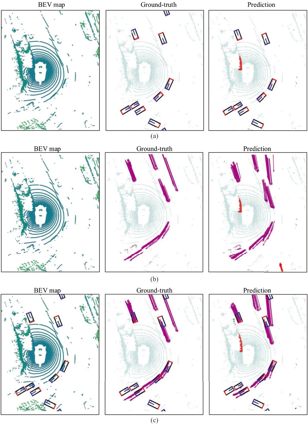
FIGURE 1(a)Shows the predicted results of a general instance‐level detector,(b)is the output of MotionNet,and(c)denotes the predicted results of the proposed ST‐SIGMA.The left images are initial bird’s‐eye view(BEV)representations,the middle ones are the corresponding ground‐truth maps,and the right images are the output of three different methods,respectively.The arrows indicate future motion predictions of the foreground grid cells,and the different colours represent different agent categories.The orientation and the length of the arrows represent the direction and distance of the agents'movement.The central area of the BEV map represents the location of the ego‐agent
To remedy the above‐mentioned issues,this paper proposes a unified scene perception and graph interaction encoding framework,ST‐SIGMA,consisting of the scene semantic encoder(SSE),graph interaction encoder(GIE),and HAD.SSE takes multi‐sweep LiDAR data in BEV as the input to extract high‐level semantic features,and GIE utilises agents'previous state information to encode graph‐structured interactive relations between neighbouring traffic agents.Then,both output features are propagated into HAD for pixel‐level prediction tasks.Notably,our model captures features of both the scene and interaction to compensate for the deficiencies in prior work.
In summary,the contribution of this paper is threefold:
·An iterative aggregation network is developed as the SSE,which iteratively aggregates shallow and deep features to preserve as much spatial and semantic information as possible for multi‐task dense predictions.
·An attention‐based feature fusion method is designed to efficiently fuse the semantic and interaction encoding features to facilitate multimodel feature learning.
·The proposed ST‐SIGMA framework can learn scene semantics and graph interaction features in a unified framework for pixel‐level scene perception and trajectory forecasting.
The rest of this paper is organised as follows:Related work is discussed in Section 2.Details on the proposed scene perception and trajectory forecasting framework are presented in Section 3.The experimental results and analysis on the nuScenes[21]data set are presented in Section 4.And finally,Section 5 draws the conclusion and the future work of this paper.
2|RELATED WORK
This section revisits some of the key works that have been proposed for scene perception,graphical interaction representation,and trajectory prediction,respectively.We also illustrate the similarities and differences between the proposed ST‐SIGMA and other works.
2.1|Scene perception
The canonical scene perception task targets the identification of the location and class of objects.According to the input modality,this task is categorised into 2D object detection,3D object detection,and multimodal object detection.2D object detection includes two‐stage methods[22],single‐stage methods[23],and transformer‐based methods[24].With the increasing adoption of LiDAR in AD,3D object detection has recently gained increasing attention.The voxel‐based method voxelizes irregular point clouds into 2D/3D compact grids and then adopts 2D/3D Convolutional Neural Networks(CNNs)[6,25].The point‐based method leverages permutation invariant operators to abstract features from raw points[26,27].Due to the ambiguity of single modality,fusion‐based object detection is emerging to address this drawback[28,29].Specifically,our method follows the pipeline of multimodal object detection,where we leverage LiDAR point clouds and graph interaction data to perform both pixel‐level categorisation and instance‐level object detection.
2.2|Graph interaction representation
Graph convolutional networks(GCN)[30]can model the dependencies between graph nodes and propagate neighbouring information to each node.It is receiving more attention in many vision tasks[31,32].ST‐GCN[33]applies to construct a sequence of skeleton graphs for action recognition,where each graph node corresponds to a joint of the human body.Refs.[34,35]use ST‐GCN to learn interaction features from human trajectories in the past and then design a time‐extrapolator CNN for future trajectory generation.Weng et al.[9]propose a graph neural network‐based feature interaction mechanism that is applied to a unified MOTand forecasting framework to improve socially aware feature learning.However,none of these trajectory prediction methods fully consider the direct or indirect interactions between traffic participants.Instead,the proposed ST‐SIGMA explicitly explores the interaction relationships between multiple traffic agents in AD scenes by leveraging ST‐GCN as a GIE.
2.3|Trajectory forecasting
Significant progress has been made in trajectory forecasting based on different data modalities.Fast and Furious[4]develops a joint detector,tracking,and trajectory forecasting framework by encoding an OGM over multiple LiDAR frames.MotionNet[8]and Fang et al.[36]propose a novel spatio‐temporal pyramid network(STPN)to jointly perform pixel‐level perception and trajectory prediction.Besides,parallelized tracking and prediction[9]utilises the past motion states of traffic agents in a top‐down grid map as the model input,and then the recurrent neural networks are applied to extract and aggregate temporal features as the interaction representation for motion prediction.With the development of high‐definition map(HDM)data,HDM data‐based trajectory forecasting methods receive more attention.GOHOME[37]exploits the graph representations of the HDM with sparse projection to provide a heatmap output that depicts the probability distribution of an ego‐agent's future position.THOMAS[38]leverages hierarchical and sparse image generation for multi‐agents'future heatmap estimation.Unlike these works,this paper utilises the fusion of the scene and interaction features for pixel‐level trajectory forecasting.
3|PROPOSED METHOD
We aim to perform simultaneous multi‐agent scene perception and trajectory forecasting in the 2D space of BEV.First,the BEV representation of the point cloud is fed to the SSE network for scene semantics encoding.Meanwhile,multi‐agent past trajectories are fed to the GIE network for interactive graph encoding as well.Then,the HAD network further fuses the features from SSE and GIE to perform scene perception and trajectory forecasting.The overall ST‐SIGMA framework is illustrated in Figure 2.Section 3.1 describes the BEV representation process.Section 3.2 presents details about scene information manipulation and the semantic encoder building process.Section 3.3 introduces motion state data preparation and explains how the graph interaction is modelled,given agents'past trajectories.Section 3.4 gives the deep aggregation decoder construction and configuration and elaborates on the rationale of network design.
3.1|BEV representation

FIGURE 2 The proposed scene perception and trajectory prediction framework,ST‐SIGMA,consists of three essential modules:SSE,GIE,and HAD.Each of them plays its own unique role for scene semantics encoding,graph interaction encoding,and feature fusion,please see the corresponding sections for details.GIE,graph interaction encoder;HAD,hierarchical aggregation decoder;SSE,scene semantic encoder;ST‐GCN,spatio‐temporal graph convolution network;ST‐SIGMA,Spatio‐temporal semantics and interaction graph aggregation for multi‐agent perception and trajectory forecasting
To make the raw point cloud from the LiDAR sensor structured and compatible with the network input,we need to transfer raw point clouds into BEV maps.Concretely,the origin of the coordinate system for each point cloud sweep changes over time due to the movement of LiDAR mounted on the ego‐agent,which leads to plausible motion estimation.To alleviate these issues,following Ref.[8],we first synchronise all the past point frames to the current coordinate system for coordinate alignment.Then wespecify the range of scene regionfrom the raw3D cloud point at timestampt,denoted as Mt∈RLc×Wc×Hc,whereLc,WcandHcdenote the length,width,and height,respectively.The origin is located at the position of the ego‐agentP0=[x0,y0,z0]by specifyingP0as the origin of synchronised coordinate system.The valid range of scene Mtw.r.tP0can be represented by,whereH0is the vertical distance from the LiDAR sensor to the ground.Thereafter,the Mtis voxelised with a predefined voxel size[δl,δw,δh]into a discretised grid mapItwith a size of.We simply encodeItas a binary BEV map.In particular,a voxel occupied by the point cloud is assigned a value of 1;otherwise,it is assigned as−1.The binary mapItis taken as the input into the SSE network for scene semantics encoding.
3.2|Scene semantic encoder
In the STPN of the baseline,we observe that pyramidal connections are linear,and the shallower layers’features are not sufficiently aggregated to mitigate their inherent semantic weaknesses.Instead of STPN,we propose SSE for progressive spatio‐temporal feature aggregations inspired by Ref.[39].Concretely,SSE takes a set of sequential BEV mapss={st|t=−T,…,−1}∈RT×Z×X×Yas the input,whereTis the number of BEV maps,andZ,XandYdenote the number of channel(height),Xaxis andYaxis of each map.The network consists of five spatio‐temporal convolution(STC)blocks.The first STC block,STC‐0,extents height channels fromZtoCwhile reserving the map resolution.The remaining four blocks double the number of height channels and reduce the resolution by a factor of two at each stage to model high‐level semantic features.The output scene semantic feature maps S∈R16C×X∕16×Y∕16are then fused with graph interaction features G(detailed in Section 3.3)to compose the semantic and interactive aggregations as the final encoding features A,which are further propagated into the decoder network with multiheads.At the same time,to preserve as much of the spatial information of the low‐level features as possible for better resolving the pixel‐level information for fine‐grain output tasks,we apply iterative aggregation connections,which are compositional and non‐linear,and the earlier aggregated layers pass through more aggregations.The iterative aggregation functionIaggregates the shallow and deep features from a series of layers{l1,…,ln},which is formulated as follows:
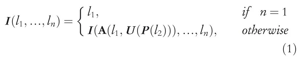
whereAis the aggregation node.Our SSE network has four iteration levels and six aggregation nodes.Each nodeAaccepts two input branches:the first branch is from feature maps that share the same resolution as aggregated features;the second branch is the feature maps down‐sampled from the first input branch.For dimension and resolution adaptation,the features of the second branch are fed into a projection blockPand an up‐sampling blockU.The projection functionPprojects the feature map channel of stage 2–6 to the number of 16,and then the un‐sampling functionUup‐samples the projected feature maps to the same resolution as the features of stage 1(256×256).The up‐sampled features are taken as input to aggregation nodeAin Equation(1).The SSE network is shown in Figure 3.
3.3|Graph interaction encoder
Besides scene semantic information,the interaction relationships between agents will influence their future trajectory in the BEV map.In general,the past motion states of an agent directly or indirectly affect its own and its neighbours'future trajectories.Therefore,we extend the GCN to the ST‐GCN to encode the graph interaction between agents,as shown in Figure 4.
To emphasise the difference from the original GCN,we revisit the preliminary knowledge of the graph convolution network(GCN),and the original GCN is formulated as follows:
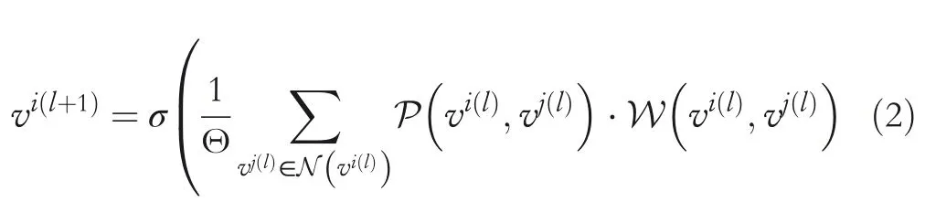
where P is the sampling function aggregating the information of neighbours aroundvi,and the superscript(l)denotes layerl.W is the learnable parameters of graph model,is a normalisation term,and Θ is the cardinality of the neighbour set.
Given multi‐agent's motion state vectorfor agentiat timestampt,it serves as the initial input of the first layer(layer0)of GIE.Here,a set of sequential motion state vectorvitfrom timestamp−Tto−1 compose the input of GIE,denoted as,whereMis the number of agents andDmeans the feature dimension for each graph node.General graph convolution networks consider only single‐frame graph representationGt=(Vt,Et),whereVt=is the set of vertices of the graph,andis the set of edges betweeni‐th andj‐th vertex.We assume that there is an edge betweenvitandvjtif theL2distance between them is less than a predefined thresholdd.To better encode the mutual interaction between neighbouring agents,each edge is weighted by a kernel functionkij
t,defined as follows:

where‖·‖is theL2distance from BEV between thei‐th andj‐th vertex,which means thatifvitandvjtare connected,andeijt=0 otherwise.Allkijtform the adjacency matrixAtof graphGt.To ensure a proper GCN,the adjacency matrixAtis normalised with identity matrixIand the degree matrix Λ as follows:

Similar to Refs.[33,34],ST‐GCNs define a new spatio‐temporal graphGconsisting of a sequential subgraphs asG={Gt|t=−T,…,−1},and allGtshare the same topology but vary vertex attributes ofvtwith a different timestampt.Thus,the graph is defined asG=(V,E),in whichV={vi|i=1,…,M},and.It means that each vertex ofGconsists of the temporal aggregation of spatial node attributes;in this way,the temporal information is naturally embedded in graphG.In addition,the normalised adjacency matrixAis the stack of{A−T,…,A−1},in whichAtis calculated as Equation(4).The vertices'representation of layerlat timestamptis denoted asV(l)t,andV(l)is the temporal stack of.Our final ST‐GCN layers is formulated as follows:
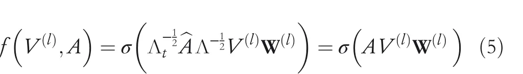
where W(l)is the learnable parameters at a laterl.After N‐layer graph convolution operation,the ST‐GCN outputs final graph feature mapsV(N),denoted as graph interaction embedding G,which is further fused with scene semantics encoding S and is then taken as input to the HAD network for dense prediction tasks.
3.4|Hierarchical aggregation decoder
Given the scene semantic feature maps S output by SSE and graph interaction feature maps G output by GIE,the proposed hierarchical aggregation decoder network takes S and G as input for simultaneous multi‐layer feature aggregation and heterogeneous feature fusion.Specifically,S is a stack of the multi‐scale feature maps{s(1),…,s(N)},s(n)is the output of then‐th aggregation stage with resolution[X/2n−1,Y/2n−1],where[X,Y]is the original size of the BEV map.There are five aggregated feature maps,except the fifth‐stage featuress(5),which are directly output by the STC‐4 block and are further fused with G.The feature maps from one to four stages■s(n)■4n=1are produced by iterative aggregation operation,defined in Equation(1).As for G,the original input of GIE is theT‐sequential stack ofN‐agents'motion state matrixFor model suitability,we first transform the dimensional order of Q to∈RD×T×M.Then,the ST‐GCN feature mapsV(N)isproduced by the ST‐GCN network,given graph vertices^Q and adjacency matrixA∈RT×M×M,andV(N)is fed into a graph residual block for the graph representation aggregator(GRA),which is composed of a stack of residual convolution operations,to obtain the final graph interaction feature maps G∈RT××M,where=M=X/16.Thus,s(5)and G share the same feature resolution and can be seamlessly fused[40]after applying the ST‐GCN and GRA network.We design three fusion approaches for heterogeneous feature fusion,as shown in Figure 5,and conduct ablation study for their effectiveness comparison in Section 4.4.3.The core of the ST‐SIGMA framework lies in the HAD network,shown in Figure 3,which plays a vital role in two aspects of dense prediction tasks.First,it enables us to neatly fuse multimodal feature maps even with diverse dimensions,resolution,and channels.Second,HAD network can iteratively and progressively aggregate features from shallow to deep to learn a deeper,higher,and finer resolution decoder with fewer parameters and better accuracy.

FIGURE 3 Hierarchical aggregation decoder(HAD)and scene semantics encoder(SSE)architectures.The SSE is responsible for scene semantic feature extraction.The HAD fuses the features from the SSE and graph interaction encoder(GIE)and then performs dense predictions.STC,spatio‐temporal convolution

FIGURE 4 Graph interaction encoder(GIE),which is implemented with the spatio‐temporal graph convolution network(ST‐GCN).Generally,the ST‐GCN is the temporal stack of spatial graph representations.Please refer to Section 3.3 for more details

FIGURE 5 Three feature fusion approaches are used in our method,and C is the concatenation operation.(a)Is the concatenation‐based fusion,(b)is the addition‐based fusion,and(c)is the hybrid fusion method,which includes concatenation,addition,and attention operations.GIE,graph interaction encoder;SSE,scene semantic encoder
3.5|Loss function
The proposed HAD network generates final feature map F∈RZ×X×Y,andZ,X,Yare the channel,width,and height of feature maps,followed by three prediction heads for object detection,pixel‐level categorisation,and trajectory forecasting,respectively.Feature maps F are first taken as input into bottle neckconv2dfor feature adaptation.Each task is supervised by following three loss functions.
Forobject detection loss,we apply the cross‐entropy loss(CE)for box classification,which is defined as follws:
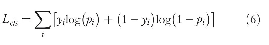
whereyidenotes the ground‐truth label of thej‐th sample,yi=1 means the foreground,andpiis the probability belonging to the foreground predicted by the learnt model.For bounding box regression,we employ a linear combination ofl1‐norm loss and the generalised IoU lossLGIoU[41].The final regression loss can be formulated as follows:
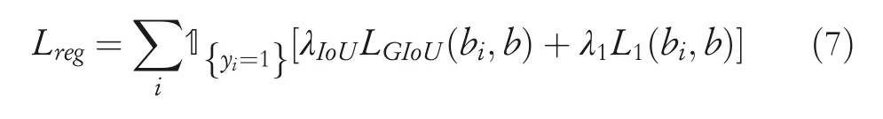
where 1{yi=1}is an indicator function for the positive sample,biis thei‐th predicted bounding box,andbis the ground‐truth bounding box.λIoUandλ1are the regularisation parameters.
Forpixel‐level categorisation loss,we employ the focal loss(FL)[42]to handle the class imbalance issues,which is defined as follows:
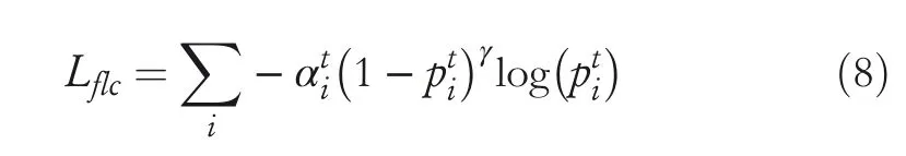
wherepti=piifyi=1,andpti=1−piotherwise,piis the predicted probability that thei‐th pixel belongs to the foreground category,andyiis the ground‐truth category labels;interested readers can refer to related literature[42]for more details.
Fortrajectory forecasting loss,with the analysis in Ref.[45],we employ a weighted smoothL1loss functionLtffor trajectory forecasting,where the weight setting follows that of the categorisation loss.However,the above loss can only guarantee the global normalisation of training and cannot guarantee the local spatiotemporal consistency.Therefore,we additionally adopt the spatiotemporal consistency loss to augment spatiotemporal consistency learning,which is defined as follows:

In Equation(9),‖·‖is the smoothL1loss,bkis the object instance with indexk,and∈R2and∈R2are the predicted displacement values of position(i,j)and position(i′,j′)at timet,respectively.It assumes that the motion states of all pixels within an instance box should be very close to each other without much jitters,referred to as spatial consistency.Similar to spatial consistency,the predicted motion states of each agents:,denoted as the average movements of all included pixels,should be smooth without large displacement changes during a short time durationΔt,whereKis the number of cells,andβtcandβscrepresent weight parameters of the temporal‐and spatial‐consistency loss,respectively.
The overall loss function of the ST‐SIGMA model is the weighted sum of above multi‐task losses,which is defined as follows:
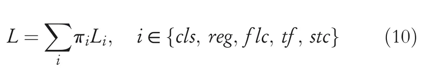
whereLclsandLregare computed for instance detection loss,LflcandLstcare formulated as pixel‐level categorisation and trajectory forecasting losses,andπiis the trade‐off parameters for balancing the multi‐task learning.
4|EXPERIMENTS AND ANALYSIS
In this section,we evaluate the performance of the proposed ST‐SIGMA method on the nuScenes data set.First,we give an introduction to the data set.Second,the implementation details and the evaluation criterion are presented.Then,we give the details of experimental analysis and compare the proposed method with existing SOTA methods.Finally,we demonstrate the effectiveness and efficiency of each module through comprehensive ablation studies.
4.1|Training and test data set
We use the nuScenes data set for all our experiments and evaluation.The nuScenes data set provides a full suite of sensor data for autonomous vehicles,including six cameras,1 LiDAR,5 mm wave radars,as well as Global Positioning System and Inertial measurement unit.It contains 1000 scenes with annotated samples,each of which is sampled within 20 Hz and contains various driving scenarios.Because nuScenes only provides the 3D bounding boxes for point clouds object detection and does not provide motion or trajectory information,we obtain the motion states between two adjacent frames by calculating the displacement vector of corresponding point clouds within the labelled bounding boxes based on theirX–Yaxis coordinate values and the displacement relative to their centre positions.For point clouds outside the bounding box,such as the background,road,roadside building etc.,the movement values are set to zero.At the same time,we crop the point clouds,and set the range on thex‐axis to be 32 m for the positive and negative axis,respectively,and the same range on they‐axis.On thez‐axis,we take into account that the LiDAR sensor is mounted on top of the vehicle,so the negative axis direction is set to 3 m and the positive axis is 2 m.
4.2|Implementation details
The size of scene range Mtis set as[−32,32]×[−32,32]×[−3,2]m3,and then Mtis discretised by the voxel size[0.25,0.25,0.4]into a grid mapItof size[256,256,13].We use five temporal frames of synchronised point clouds as SSE network inputwith tensor size 5×13×256×256.We define five categories for instance‐level classification and pixel‐level categorisation prediction,for example,vehicle,pedestrian,bicycle,background,and others.The‘other’category includes all the remaining objects in nuScenes to handle the possible unseen objects beyond the data used in our paper.For the GIE network,we use 8‐dimension motion vectorsfor each traffic agent,whereand each quantity containsx‐axis andy‐axis components.For spatial‐temporal graphG,we construct network inputwith size 5×8×20×20,which are generated from the same five temporal frames with the input of SSE.And the SSE encoder outputs scene semantic features S,GIE outputs graph interaction features G,and both of them share the same size 32×16×16.Then,we apply three feature fusion approaches to fuse them,that is,channel‐wise concatenation,channel‐wise addition,and attention‐augmented addition.And we further verify their effectiveness in the ablation studies.The visualisation of predicted results by ST‐SIGMA is shown in Figure 6.
4.3|Evaluation criterion
For trajectory forecasting,we calculates the relative displacements of the corresponding point clouds in adjacent frames.Meanwhile,all grid cells within BEV map are classified into three groups according to their moving speed,for example,static,slow(speed≤5 m/s),and fast(speed>5 m/s).In each group,the averageL2‐norm distance between the estimated displacement and the ground truth displacement,that is,the average displacement error(ADE),is calculated in Equation(11):

In Equation(11),Nrepresents the number of traffic agents,represents the predicted trajectory of then‐th traffic agents at timestampt,andrepresents the true trajectory,wheret=1,…,Tfuture.Equation(12)computes the Overall cell category Accuracy(OA)of all cells,formulated as follows:

where Correct classified Cells(CC)represents the number of correctly classified cells,and AC represents the total number of cells.And Equation(13)calculates the Mean Category Accuracy(MCA),which indicates the average category accuracy:

where CA(Bg)represents the classification accuracy of the background,CA(Vehicle)represents the classification accuracy of vehicles,CA(Ped)represents the classification accuracy of pedestrians,CA(Bike)represents the classification accuracy of bicycles,and CA(Others)represents the classification accuracy of other unseen traffic objects,respectively.
4.4|Experimental analysis

FIGURE 6 The visualisation of predicted results by each head,for example,the predicted pixel categorisation(using different colours to represent different categories),bounding boxes,and the trajectories of traffic agents
We evaluate the performance of our proposed ST‐SIGMA method and compare it with other SOTA perception and trajectory forecasting methods.Specifically,for pixel‐level categorisation and trajectory forecasting,we compare with the following methods:static model,which only considers the static environment;FlowNet3D[43],HPLFlowNet[44],Neural scene flow prior[46]and recurrent closest point[47],which estimate the scene flow between adjacent point cloud frames with linear dynamic assumption;PointRCNN[27],which is the combination of the PointRCNN detector and Kalman filter for bounding box prediction and trajectory forecasting of objects in BEV representation;LSTM‐Encoder–Decoder[45],which estimates the multi‐frame OGMs by using the same prediction head as ST‐SIGMA while preserving its backbone network;and MotionNet[8],which adopts LiDAR point clouds and the STPN framework for scene perception and motion prediction.It is noteworthy that our ST‐SIGMA is inspired by the baseline[8],but with three novel contributions.First,we discard the STPN backbone and replace it with the iterative aggregation network,which can better propagate low‐level features to high‐level stages for multi‐scale feature aggregation.Second,we employ a GIE to further learn interactive relations between traffic agents.Third,we introduce an additional instance‐box prediction head for instance‐level object detection,which can directly boost pixel categorisation performance by capturing higher‐level semantic information from traffic scenes.For evaluating the performance of the bounding box prediction,we compare our method with SOTA detectors,including PointPillars[6],PointPainting[29],shape signature networks[48],Class‐balanced grouping and sampling[49],and CenterPoint[14].Moreover,we further compare the complexity of the proposed ST‐SIGMA with different scene perception and trajectory forecasting methods.
4.4.1|Quantitative analysis
To better evaluate the performance of the proposed method in different traffic scenarios,we first divide all the grid cells into 3 groups by different moving speeds:static(velocity=0 m/s),slow(velocity≤5 m/s),and fast(velocity>5 m/s).As shown in Tables 1–5,the ST‐SIGMA‐Baseline adopts the STPN backbone network proposed by the baseline method to extract scene semantic features from the BEV representation,and is additionally equipped with GIE.ST‐SIGMA employs the iterative aggregation network instead of STPN,and includes SSE,GIE,HAD,and the attention‐based fusion.
From Table 1,we can see that for static cells,the static model gets the best trajectory forecasting performance,but the ADE increase with the moving speed of grid cells,which means the static model only performs well under extreme conditions and is not suitable for real‐world and dynamic AD scenes.A similar phenomenon happens to FlowNet3D[43],HPLFlow-Net[44],and PointRCNN[27];all of them achieve good prediction results for static cells;however,their performance drops dramatically for moving objects.Unlike the above methods,MotionNet[8]has a fairly stable model performance and shows the excellent performance for slowly moving objects;it outperforms all other methods including ours when moving velocity≤5 m/s.Instead,our proposed ST‐SIGMA method yields the best performance for fast moving objects.Specifically,it outperforms MotionNet by 0.0217 in terms of ADE,and 0.0637 in terms of median displacement error,respectively.This superiority is attributed to the graph interaction features,which can effectively model dynamic interactive relations,especially for the fast‐moving traffic agents with velocity>5 m/s.In addition,we can draw the conclusion that each component(SSE,HAD,and feature fusion approaches)plays a positive role for performance improvement.Notably,ST‐SIGMA with the attention‐based fusion approach achieves the best performance of trajectory forecasting,which suppresses the baseline by 2.3%,please refer to Tables 1 and 5 for more details.
For evaluating pixel categorisation performance,we apply two types of loss functions:CE and FL.As shown in Table 2,ST‐SIGMA+ALL+CE denotes ST‐SIGMA with CE loss,and ST‐SIGMA+ALL+FL denotes ST‐SIGMA with FL function.We compare the proposed method with PointRCNN,LSTM‐Encoder–Decoder,and MotionNet.Table 2 demonstrates that across all five categories,the proposed ST‐SIGMA achieves the highest accuracy for four foreground categories,that is,car,pedestrian,bike,and others.We consider MotionNet as the baseline method;for CE,ST‐SIGMA increases categorisation accuracy by 1.5% compared to the baseline method.When applying FL,it further improves the performance of the baseline by 1.8%.For the pedestrian category with a small sample size,our method receives a significant performance improvement.Specifically,it increases the categorisation accuracy from 77.2 to 83.8,which outperforms the baseline method by 6.6%.For‘others’foreground categories,whose categorical information are not specified in this paper,ST‐SIGMA still achieves much better accuracy than the baseline by more than a 10%performance improvement.And the MCA of ST‐SIGMA is 75.5,which is 4.4%higher than that of the baseline.Notably,there is no obvious performance improvement for the background category and the overall cell categorisation.We analyse that for most point cloud frames,the point clouds belonging to the background category is much more than foreground point clouds.Once we use multi‐frame BEV maps to get the temporal‐aggregated scene features,these aggregated features can facilitate the detection of the foreground object with a small number of point clouds,but for the background category with a large number of point clouds,iterative aggregation network may cause over‐fitting issues due to over‐aggregation of background features.We will address this issue in a future study.
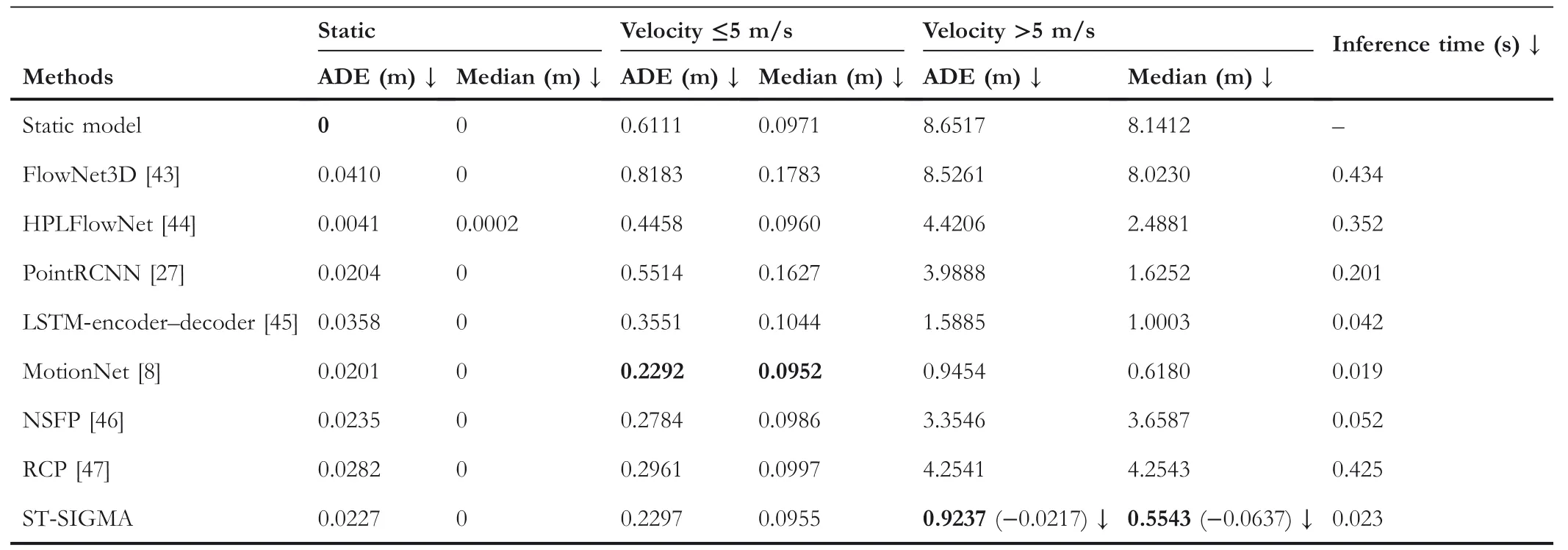
TABLE 1 In the comparison of trajectory forecasting performance,we compare ours with some state‐of‐the‐art methods

TABLE 2 The comparison of pixel‐level categorisation performance
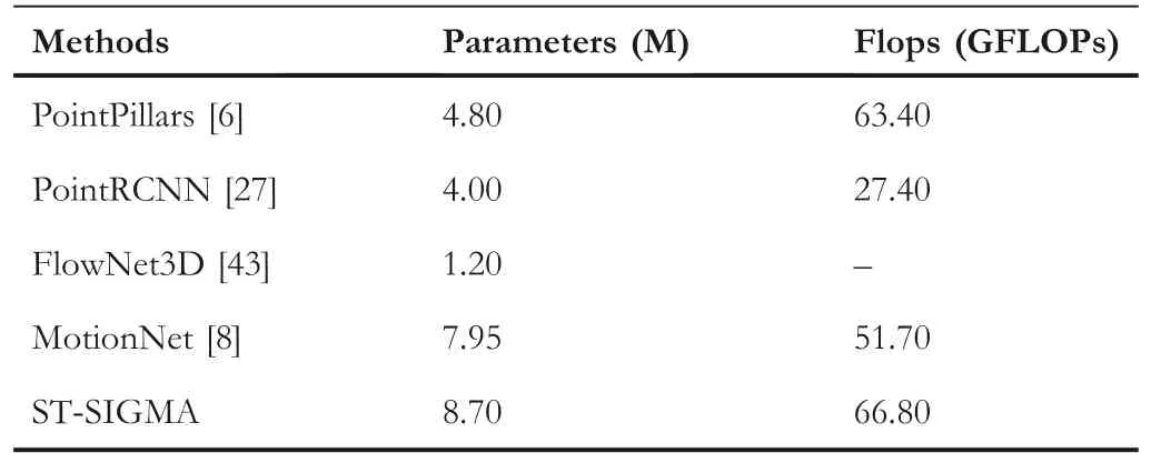
TABLE 3 The complexity comparison of the proposed ST‐SIGMA and some state‐of‐the‐art scene perception and trajectory forecasting methods
Besides dense pixel‐wise predictions,we additionally add an instance‐level detection for the object bounding box prediction,as shown in Table 4.We compare the performance of ours with the most commonly used 3D object detectors.Our detector is based on the aggregated BEV maps and only performs 2D detection,although the performance of ST‐SIGMA is far inferior to most of SOTA 3D detectors,such as CenterPoint.However,employing this detection function can help to disambiguate the pixel categorisation process by providing both the spatial consistency constraint and the additional semantic information.To further evaluate the efficiency of the proposed method,we further compare the complexity of ST‐SIGMA with the following methods,PointPillars[6],PointRCNN[27],Flow-Net3D[43]and MotionNet[8].Table 3 shows that the complexity of the proposed ST‐SIGMA is about 10% higher than that of the baseline method.We attribute the complexity growth to the usage of multimodal data input and the iterative network architecture.
4.4.2|Qualitative analysis
To qualitatively evaluate the proposed ST‐SIGMA method,we visualise predicted results of the pixel categorisation and trajectory forecasting in Figures 7 and 8,and compare it with corresponding ground‐truth maps and the predicted results of the baseline method.For the convenience of qualitative analysis,we first give the detailed description of the elements and attributes in the following figures.
Specifically,in Figure 7a,there are five different colours of point clouds;different colours denote the different categories of traffic agents,for example,blue points represent the background,purple points mean vehicles(cars or truck),black points mean the pedestrian,green points denote the bicycle,and red points mean other foreground categories.In Figure 7b,besides point clouds,there are five different colours of arrows,where each colour represents the category information that is the same with points,and the arrows represent the future trajectory of each point.Concretely,the length of the arrowindicates the moving distance,and the direction of the arrow means the moving orientation.Figure 7a shows the comparison of ground‐truth maps,the predicted results of our ST‐SIGMA,and the baseline method.In pixel categorisation results,there are fewer pixels misclassified by ST‐SIGMA than the baseline,as shown in the regions enclosed by the circle.It demonstrates that the categorisation performance of the proposed method is better than that of the baseline.As for trajectory forecasting results in Figure 7b,it is clear to see that the points at the bottom of the map are misclassified by the baseline,but ST‐SIGMA gives robust categorisation results thanks to the additional instance detection function.More visualisation of trajectory forecasting results are shown in Figure 8,where each row represents the comparison between ground truth,predicted results of ST‐SIGMA,and the baseline in a traffic scene.In first row,the points belonging to other category at the top of the map are misclassified into vehicles by the baseline.Instead,the proposed ST‐SIGMA can accurately categorise them.However,in the second row,for traffic agents that are too close or too far from the ego‐vehicle,our methods occasionally perform false detection,which indicates that our method has lower robustness compared to the baseline method in these traffic scenarios.
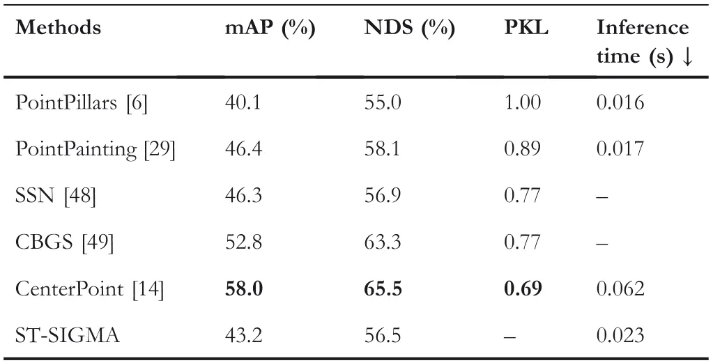
TABLE 4 The comparison of object detection performance

FIGURE 7 The pixel‐level categorisation prediction results(first row),and the trajectory forecasting results(second row),from left to right:the ground‐truth category map,the predicted results of ST‐SIGMA,and the predicted results of the baseline method.ST‐SIGMA,Spatio‐temporal semantics and interaction graph aggregation for multi‐agent perception and trajectory forecasting
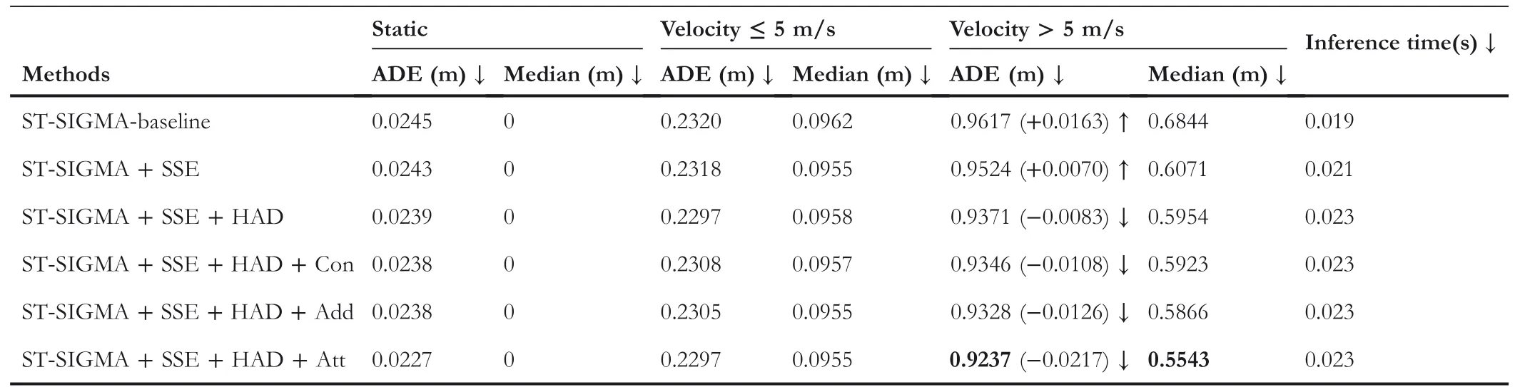
TABLE 5 Ablation study about the effect of each component on the ST‐SIGMA framework
4.4.3|Ablation study
In this section,we estimate the validity and effectiveness of each proposed component through comprehensive ablation studies.First,we focus on the proposed ST‐SIGMA framework,which consists of four key components,SSE,GIE,HAD,and feature fusion approaches(Con,Add,and Att).Table 5 shows that the ST‐SIGMA‐Baseline adopts the STPN backbone network from the baseline to model BEV maps,and is additionally equipped with GIE.In Table 5,the second row replaces STPN with the iterative aggregation network for scene semantics encoding,and leaves the rest unchanged.The third row further applies the HAD network for hierarchical multimodel feature aggregation.And the fourth to sixth rows apply Concatenation‐based fusion,element‐wise Addition‐based fusion,and Attention‐based fusion approaches,respectively.As shown in Figure 5,(a)is the Concatenation fusion(Con),(b)is the element‐wise Addition fusion(Add),and(c)is the Attention‐based fusion(Att),respectively.We can also draw the conclusion that each component plays a positive role in the performance improvement of ST‐SIGMA.If we take MotionNet as the baseline,we can see that only simply adding interaction encoding cannot help improve the trajectory forecasting accuracy.And ST‐SIGMA with the attention‐based fusion approach obtains the best performance,which suppresses MotionNet by 2.3%.
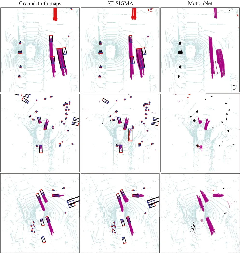
FIGURE 8 The pixel‐level categorisation prediction of three selected scenes,from left to right:the ground‐truth category map,the predicted results of ST‐SIGMA,and the predicted results of the baseline.ST‐SIGMA,Spatio‐temporal semantics and interaction graph aggregation for multi‐agent perception and trajectory forecasting
Furthermore,we analyse the effect of different weighted adjacency matrix kernel functions,which define the mutual influence between vertices and provide the prior knowledge of social relations among traffic agents.Since the graph interactions have a large impact on the future trajectory of agents,specifically,we analyse the influence of different kernel functions,k1,k2,k3,k4andk5in Equation(14),on the trajectory forecasting performance(ADE)of multiple traffic agents,and the results are shown in Table 6.
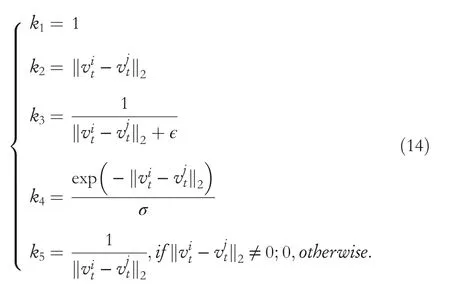
In Equation(14),we setk1=1 as the baseline in the weighted adjacency matrix.And the second kernel functionk2is defined as the Euclidean distance(L2 norm)between traffic agents to simulate their influence on each other.The third kernelk3is defined as the inverse of the L2 norm and adds a residual parameterϵto the denominator,making sure the denominator is not equal to 0.The fourth kernel functionk4is calculated using the Gaussian radial basis function[50].And the fifth kernelk5is also defined as the inverse of the L2 norm,but different fromk3,we setk5=0 in the case of,wherevitandvj
trepresent thei‐th agent andj‐th agent at timestampt.It indicates that two traffic agents are considered to be the same object when they are at the same location.The performances of these kernel functions are shown in Table 6,and through ablation experiments,we can see that the best performance is produced byk5,since the future motion of traffic agents are more sensitive to theinfluence of other similar objects physically close to them.Therefore,this study computes similarity measurements for traffic agents to address this issue.Conversely,without this condition,the relationship between traffic agents in the model cannot be correctly represented.Therefore,this paper usesk5to define the adjacency matrix in all experiments.
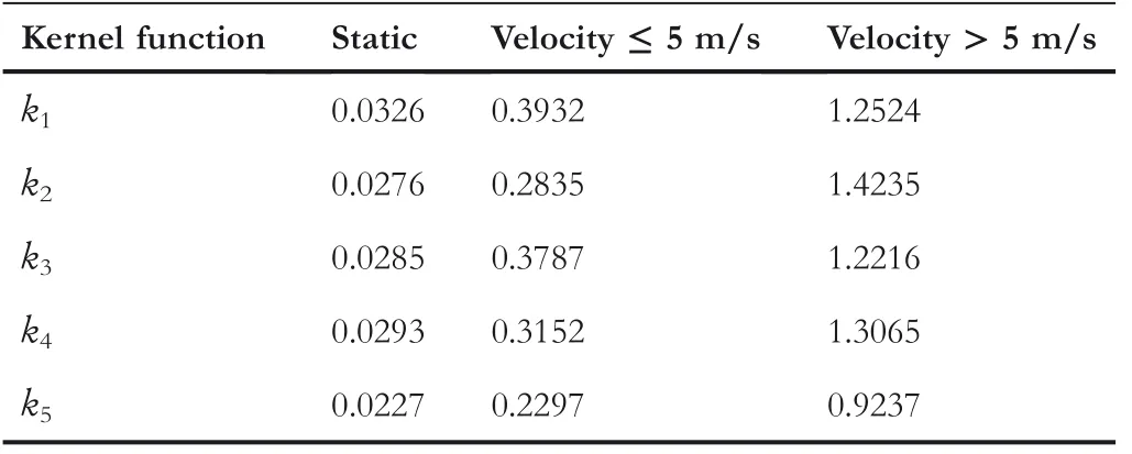
TABLE 6 Ablation analysis about the influence of different kernel functions on trajectory forecasting performance
In addition,we also try to find the optimal number of input BEV frames for trajectory forecasting performance.To achieve this goal,we draw the curve graph in Figure 9 to show the relationship between the number of input frames and the average displacement errors of trajectory forecasting.It is observed that when the number of input frames increases from 1 to 5,all ADE are consistently decreased.However,the time and space complexity will increase significantly with the increase in the input frame number.We need to make a trade‐off between the number of input frames and the model performance.As shown in Figure 9,when the number of frames exceeds 5,the model performance gradually saturates and even decreases for fast moving traffic agents.Hence,we set the number of input frames to 5 for all experiments.
5|CONCLUSIONS
This paper proposes ST‐SIGMA,a unified framework for simultaneous scene perception and trajectory forecasting.The proposed method can jointly and accurately perceive the AD environment and forecast the trajectories of the surrounding traffic agents,which are crucial for real‐world AD systems.Experimental results show that the proposed ST‐SIGMA framework outperforms the SOTA method by 2.3% higher MCA for pixel categorisation and 4.4%less ADE for trajectory forecasting.In future work,we intend to utilise multimodal data fusion(LiADR,camera,HD‐Map)and adopt traffic rules to further improve the performance of scene perception and trajectory forecasting while maintaining the acceptable complexity cost.

FIGURE 9 Ablation analysis about the effect of the number of input frames on the trajectory forecasting performance.Considering the accuracy and the efficient trade‐off,we chose 5 as the optimal number of input frames for all experimental settings.ADE,average displacement error
ACKNOWLEDGEMENTS
This work was supported in part by the Science and Technology Research Program of Chongqing Municipal Education Commission(No.KJQN202100634 and No.KJZD‐K201900605),National Natural Science Foundation of China(No.62006065),Basic and Advanced Research Projects of CSTC(No.cstc2019jcyj‐zdxmX0008).
CONFLICT OF INTEREST
The authors declared that they have no conflicts of interest to this work.
DATA AVAILABILITY STATEMENT
Research data are not shared.
ORCID
Yang Fanghttps://orcid.org/0000-0001-6705-4757
 CAAI Transactions on Intelligence Technology2022年4期
- CAAI Transactions on Intelligence Technology的其它文章
- Modelling of a shape memory alloy actuator for feedforward hysteresis compensator considering load fluctuation
- Apple grading method based on neural network with ordered partitions and evidential ensemble learning
- An improved bearing fault detection strategy based on artificial bee colony algorithm
- Parameter optimization of control system design for uncertain wireless power transfer systems using modified genetic algorithm
- Passive robust control for uncertain Hamiltonian systems by using operator theory
- Humanoid control of lower limb exoskeleton robot based on human gait data with sliding mode neural network