A Survey on the Control Lyapunov Function and Control Barrier Function for Nonlinear-Affine Control Systems

Boqian Li, Shiping Wen,, Zheng Yan, Guanghui Wen,

Senior Member, IEEE, and Tingwen Huang,Fellow, IEEE

Abstract—This survey provides a brief overview on the control Lyapunov function (CLF) and control barrier function (CBF) for general nonlinear-affine control systems.The problem of control is formulated as an optimization problem where the optimal control policy is derived by solving a constrained quadratic programming (QP) problem.The CLF and CBF respectively characterize the stabilityobjective and the safetyobjective for the nonlinear control systems.These objectives imply important properties including controllability, convergence, and robustness of control problems.Under this framework, optimal control corresponds to the minimal solution to a constrained QP problem.When uncertainties are explicitly considered, the setting of the CLF and CBF is proposed to study the input-to-state stability and input-to-state safety and to analyze the effect of disturbances.The recent theoretic progress and novel applications of CLF and CBF are systematically reviewed and discussed in this paper.Finally,we provide research directions that are significant for the advance of knowledge in this area.

I.INTRODUCTION

OVER the past several decades, affine-control systems have caught much attention from researchers and scholars due to their wide uses in the fields of science and engineering [1], [2].One essential issue of affine-control systems is to design feasible controllers that make the systems realize corresponding control objectives under different circumstances,such as the stability, safety and robustness.

Stabilityis an important property of affine-control systems and means that the system state is desired to converge to a fixed point with time under the appropriate controllers [3].System stability is usually verified by the Lyapunov Stability Theory with the help of the control Lyapunov function (CLF)[4], [5].In these recent years, the Lyapunov-like functions have been widely applied in the stabilization control for a series of systems, such as neural networks (NNs), robotic systems, nonlinear fuzzy systems, and so on [6], [7].In [8], a deep NN structure was constructed to approximate the CLF for a high-dimensional system, under which the amount of hyper-parameters was quite reduced.Additionally, in the multi-agent systems (MASs), the Lyapunov functions were widely used to demonstrate whether the designed controllers were appropriate for specific control problems, such as consensus control, formation control and containment control[9]–[11].

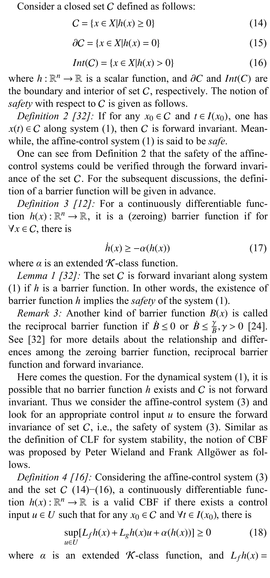
Safety, which ensures that the system state remains in a safe region during the whole control process, is another important and significant property of the affine-control systems [12].For example, in the robotic systems, safety is a fundamental requirement and needs to be considered in reality; it is also named safety-critical control [13].Zenget al.studied the safe optimal performance of avoiding obstacles for a 2-D double integrator robotic system [14].Inspired by the CLF for system stability, the control barrier function (CBF) was similarly proposed to describe the safety property of the affine-control systems [15], which was then developed in [16].The CBF has been devoted to enforcing safety for the control systems with the idea of forward invariant set [17], [18].

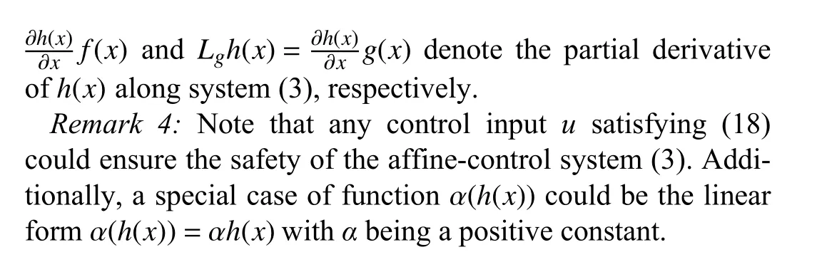
According to the above discussions, bothstabilityandsafetyare essential performances of the control systems.The study of a control system is meaningless if it is not stable, and the system safety always needs to be considered in application.In previous related studies, the common situation is to design a potential controller for the control objective at first, then verify its feasibility theoretically and experimentally, such as with state-feedback control protocol for stability [19] and a function-based control method for safety [20].However, one can see from the existing works that the appropriate controller is not unique for control systems, that is to say, more than one control input could be found to achieve good system performances.To check if a potential controller is feasible in providing stability and safety, the Lyapunov function and barrier function is commonly used, respectively.Usually, stability can be ensured with any controller that satisfies the CLF constraint and safety can be ensured with any controller that satisfies the CBF constraint.

To deal with the constraints in the control field, different control protocols have been given in the open literature, such as the model predictive control, the reference governor strategy and the invariance control principle [21], [22].In the former two control strategies, allowable reference signals were generated by a high-level controller for the low-level controller so as toavoid the constraints.In the latter strategy, the control idea was based on a switching concept and extended from the feedback control.Afterwards, some relevant works combined the barrier function and CLF to realize the stabilization objective with state constraints [23], [24].However, this kind of combination might result in the unbounded CLF around the boundary of the safe region.Therefore, a more general method was proposed to incorporate the CLF and CBF where unboundedness would not occur, which was illustrated in [25].As stated in [26], for a valid CLF or CBF, not only one control input could be found feasible for the control objectives.To help ourselves make more appropriate choices under this circumstance, the optimal controller is selected with some meaningful cost functions.A meaningful function indicates that a penalty is placed on the system state or the control input, which helps construct the optimization problems.

As an important branch of the optimization field, quadratic programming (QP) is a useful and convenient tool since the cost function is quadratic and easily solved [27].Additionally,considering that the dynamics of the affine-control systems are linear subject to the control input, the CLF and CBF constraints are also obtained with the linear forms on the control input, which fortunately fit well as the QP constraints [28],[29].The cost functions in the QP problems may vary from different targets.For example, one can minimize the control input [30], or minimize the gap between the control input and a desired controllerud[31].One can consider only one constraint in the QP problems, or consider two or more constraints.In [32], both CLF and CBF constraints were combined in the QP problem with different priority, i.e., CBF constraint was prior to CLF constraint in order to ensure the QP was solvable.The optimal controller was obtained that firstly ensured safety and secondly ensured stability.Together with the CLF, CBF and QP, the three terms help provide a control approach for the affine-control systems, under which both stability and safety (two important properties in the control field)can be ensured while the cost function has a minimum value at the same time.In order to better understand optimization control for physical scenes in our lives, the study of the CLFCBF-based QP problems for nonlinear-affine control systems deserves to be reviewed and summarized, which is the main motivation of this survey.

Considering the external disturbances and noises in the operating environment, therobustnessof CLF and CBF has been investigated for uncertain control systems [33].The disturbances might exist with different forms.For example, Alan et al.studied the case where the control input was affected by noise (during the encoding and decoding in the sensors) [34].In this case, input-to-state stability (ISS) and input-to-state safety (ISSf) were imported to describe the robustness.Zhaoet al.investigated the case where the dynamics of systems were affected with a disturbed term [35].An observer was designed for an unknown disturbance, with which the corresponding CLF and CBF were improved into robust functions.In addition, the Unscented Kalman Filter was also a potential method to apply to uncertain systems, where it was beneficial to estimate the mean and variance of the unknown disturbances [36].

Based on the above analysis, the motivations of this survey can be concluded as follows.The performance of the affinecontrol systems (such as stability and safety) is an important topic, and the study of CLF and CBF has attracted much attention and made some progress in recent years.Meanwhile,researchers have been interested in QP optimization problems and contributed increasing results.What is more, robust CLFs and CBFs have been developed in the latest years for uncertain control systems, which deserves to be summarized again.Therefore, this survey discusses the development of the CLF and CBF (Section II), introduces the different forms of QP problems (Section III), studies the robustness of the uncertain control systems (Section IV), shows the applications of CLFCBF-based QP control in the nonlinear-affine control systems(Section V), and looks at potential research directions (Section VI).What is more, Fig.1 gives an overview of this survey.

Notations:All the abbreviations of this survey are listed in Table I.Most of the notations throughout this survey are listed in Table II.In addition,I(x0)=[t0,T] denotes the time interval wheret0is the initial time instant,x0=x(t0) is the initial system state, andTis the ending time instant.For a function α:[0,a)→[0,∞) with α(0)=0 and constanta＆gt;0, ifαis continuous and strictly increasing, then it is said to be a Kclass function.For a function β:[−b,a)→(−∞,∞) with β(0)=0 and constantsa,b＆gt;0, ifβis continuous and strictly increasing, then it is said to be an extended K-class function.

II.SYSTEM MODELS AND PROBLEM DESCRIPTION

This section will introduce the notions of affine-control systems, system stability and CLF, system safety and CBF,higher relative degree and exponential CBF.

A.Affine-Control Systems

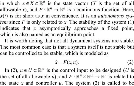
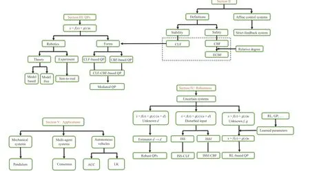
Fig.1.An overview of this survey.

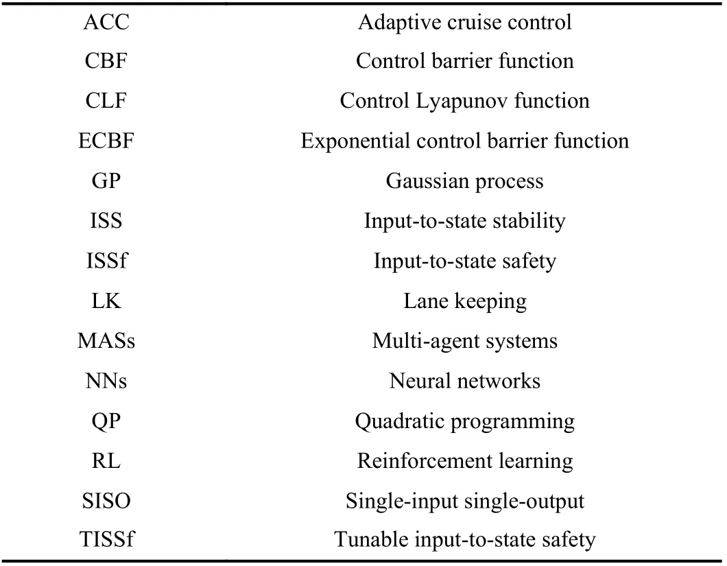
TABLE I LIST OF ABBREVIATIONS THROUGHOUT THIS SURVEY

Consider a system with the following dynamics:affineifFis linear subject to controlleru, i.e.,

wheref:Rn→Rnandg:Rn→Rn×mare related toxand independent ofu.What is more, iff,gare nonlinear functions,(3) is said to be a nonlinear-affine control system [37].Remark 1:Take the strict-feedback nonlinear system as an example.As a type of nonlinear-affine control system, the strict-feedback system only depends on the states that are feedback to the subsystem, which is described as

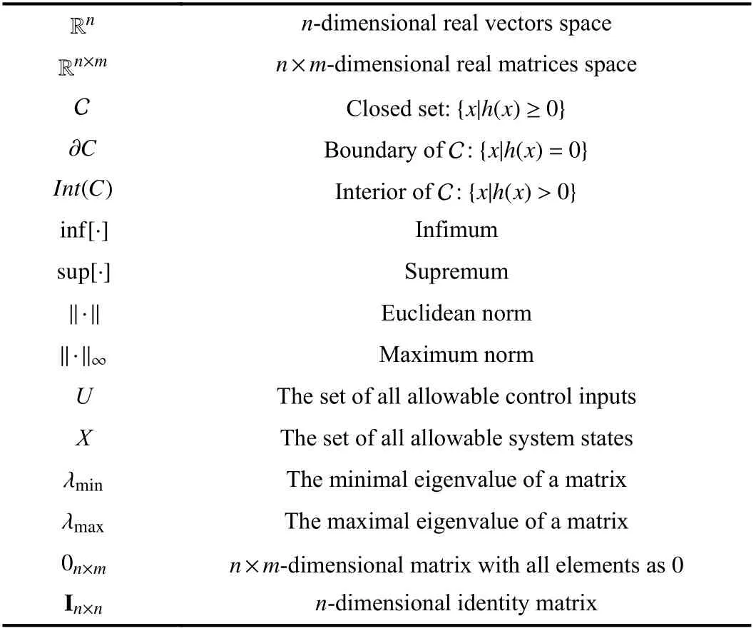
TABLE II LIST OF NOTATIONS THROUGHOUT THIS SURVEY

wherei=1,...,n−1,x=[x1,...,xn]∈Rnis the state vector,y∈R is the system output, andfj,gj(j=1,...,n) are nonlinear smooth functions.In the early stage of the study, an adaptive back-stepping control protocol and a recursive design method were used to achieve stability or asymptotic tracking objectives for strict-feedback systems [38].The back-stepping technique was further extended in strict-feedback systems with unknown control parameters and robust controllers were also studied in [39], [40].Afterwards, combined with the back-stepping strategy, the NNs were introduced in the adaptive control of the strict-feedback nonlinear system (4), which made it very suitable for parallel processing in actual applications [41].After that, the event-triggering approach was applied in the control of system (4), which could sample the state and reduce the update frequency of the NN weights [42].Note that only part of the open literature is listed here, and more control protocols deserve to be studied for the affinecontrol systems.

B.Stability and CLF

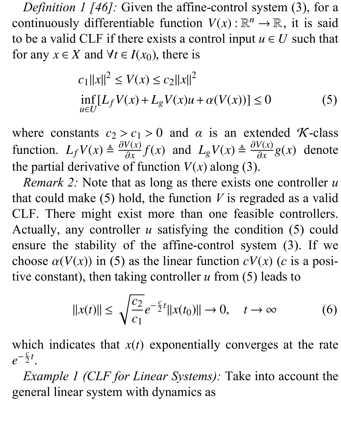
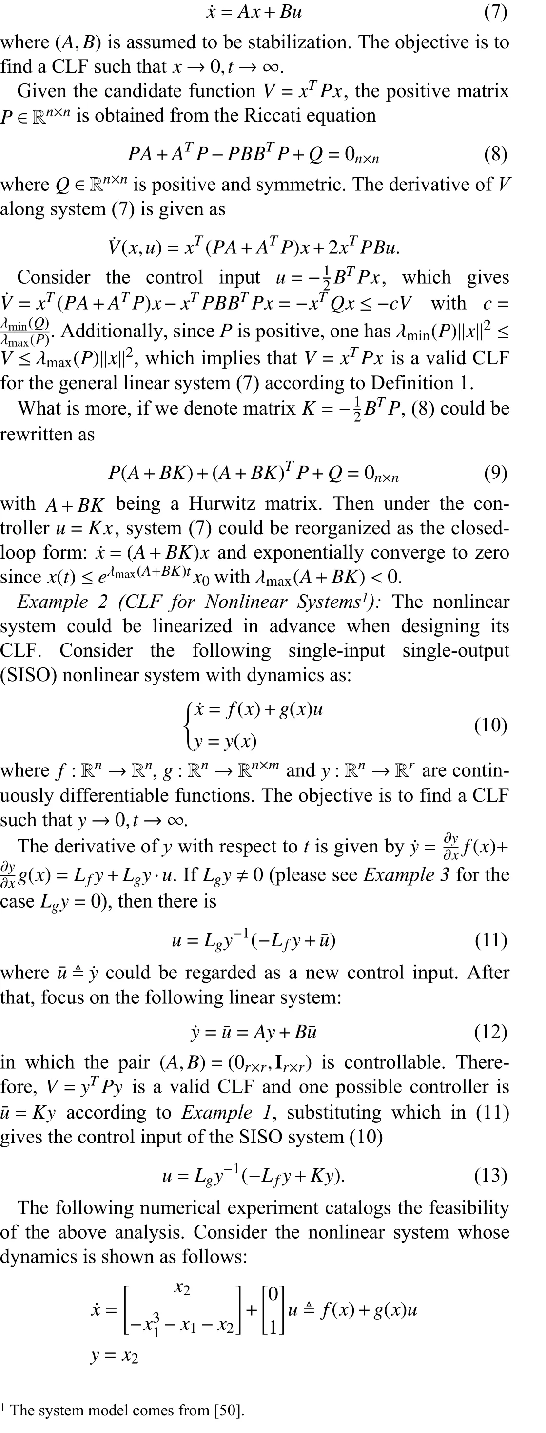
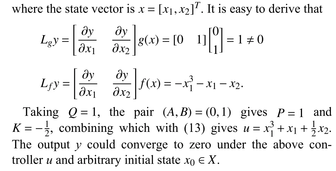
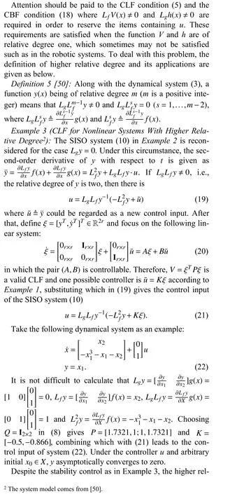
System stability is usually verified by the Lyapunov Stability Theory, which means that a positive Lyapunov functionV(x) has the derivativeV˙(x)≤0.IfV˙(x)≤−cV(x),c＆gt;0 is satisfied, the dynamical system (1) is said to be exponentially stable or exponentially convergent [43].The conclusion is similar for the control system (2).Given a control inputu, the negative ofV˙(x) along (2) can verify its capability of rendering the system asymptotically stable, which has been widely applied in the recent years [44], [45].The notion of CLF was firstly proposed in [46] and generalized in [47], which had been associated with some cost functions known as optimal control problems [30].The CLF-based linear quadratic optimal control for nonlinear systems was studied by Freeman and Primbs [26], which inspired a large volume of published studies of optimization problems for the affine-control systems[48], [49].Before moving onto the main topic of this survey,the definition of CLF is introduced as follows.

C.Safety and CBF

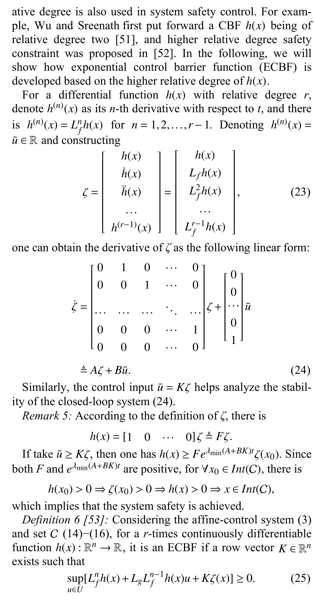
D.Higher Relative Degree and ECBF

III.QP FOR AFFINE-CONTROL SYSTEMS

Quadratic programming contributes to facilitate a kind of optimal controller based on CLF and CBF constraints to respectively depict the stability and safety performance of affine-control systems.Combined with different cost functions, QP may give solutions to different situations.This section will introduce and compare some of them.

A.CLF-CBF-Based QPs

Freeman and Kokotovic studied the min-norm controller under CLF-based QP framework [30], which is shown as follows:

The objective is to minimize the norm of controlleru∗while maintaining system stability.If safety is required, the CBF constraint could be imported in the QP framework and the cost function could also be extended to the following form:

However, it is worth noting how to determine that there exists a solutionu∗to the CLF-CBF-based QP (28).The two constraints might be conflicting such that no control inputuexists to ensure both system stability and safety.Thus, the more important one needs to be chosen from the two performances.Ames et al.mediated the specifications in [32].For example, safety is usually the necessary requirement in robotic systems, which should be regarded as ahardconstraint.While stability could be a little relaxed as asoftconstraint.In this case, the QP problem (28) is extended to the following form:

where u ∈Rm+1,H(x)∈R(m+1)×(m+1),F(x)∈Rm+1andδis a positive constant.The parameterδindicates that safety performance comes prior to the stability, under which the existence of the solution to the QP (29) is given as follows.

Lemma 2 [32]:For the affine-control system (3) and QP(29), assuming that functionsf,g,H,F, and the gradients of the CLFVand CBFhare all locally Lipschitz, ifLgV(x)≠0 andLgh(x)≠0 (i.e., relative degree one) hold for anyx∈Int(C), then the CLF-CBF-based QP problem (29) has a locally Lipschitz continuous and unique solution u∗.

If the assumption ofLgh(x)≠0 is not satisfied, one can extend to the more general case with a higher relative degree,to help construct the following CLF-ECBF-based QP problems:

Different from the QP (29), Gurrietet al.proposed the following formulation to seek a safe controlleru∗near a (potentially) unsafe controllerudwith minimum cost [54]:

Remark 6:The solution to the QP (31) is the nearest controller aroundudto maintain the system safety [55], [56].Compared with (29) and (31), consider the situation where the desired controllerudis pre-designed to ensure stability such as the state-feedback controller, but violates the safety requirement.Since safety is thehardcondition, the CBF constraint is reserved in the QP formulation.At this moment, the effect of the CLF constraint in (29) has been described byudand embedded in the cost function of (31), which has the similar meaning with the relaxation parameterδ.Taking the general linear system (7) as an example, the controllerud=Kxensures system stability, with which the QP (31) allows for the optimal controller to render system safety in a minimally invasive way.Additionally, Fig.2 shows the flowchart of the QP controller (31).

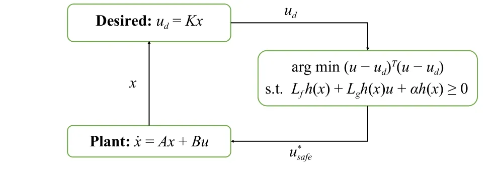
Fig.2.A structure of the QP (31).

B.QPs in Robotic Systems

In this section, we specific the nonlinear-affine control systems as the robotic systems, whose dynamics could be described as

whereq∈Rnis the configuration state,q˙ is the robot velocity,D(q)∈Rn×nis the inertia matrix,C(q,q˙)∈Rn×nis the Coriolis matrix andG(q) is the gravity matrix.If the system parametersD(q),C(q,q˙),G(q) andBare known, it is convenient to constructu, which is known as a model-based controller.Otherwise, if they are unknown, then the designeduwithout these system information indicates a model-free controller.

1) Model-Based Controller

The robotic system (32) could be rewritten as

Invoking the same outputy(q,q˙) as in [57] which is of relative degree two, the second derivative ofyis calculated as

SinceLgLfy(q,q˙) is invertible and if the system parameters are known, one can obtain the model-based controller asu=(LgLfy)−1(−L2fy+v)=−(LgLfy)−1L2fy+(LgLfy)−1v, wherevis solved from the following CLF-based QP problem:

The output (33) is not only useful for the robotic systems,but also for the nonlinear-affine control systems with relative degree 2, which is calledinput-output linearization.What is more, the structure of the QP (34) can be found in Fig.3.

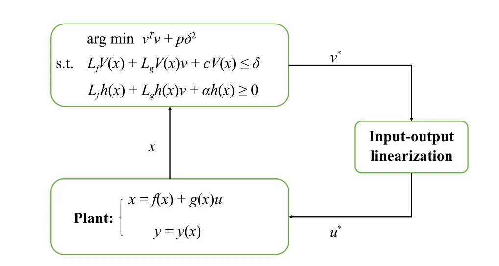
Fig.3.A structure of the QP (34).

2) Model-Free Controller

The example in [31] is introduced here to better describe the model-free controller when the system parameters are unknown.Molnaret al.considered velocity tracking control for the robotic system (32), where the control objective was to reach the destination position while avoiding the obstacles.Shown in Fig.4, the goal was to enforce the system stateqtraveled from the staring pointq0to the ending pointqg.Obviously, the originally desired velocity could beq˙d=−K(q−qg).However, an obstacle was considered and depicted as a circle with pointObeing the center andrbeing the radius.Thus the safe set was given as

Due to the existence of the obstacle,q˙dmight be unsafe.To deal with the problem, the CBF-based QP was applied to obtain the safe velocityq˙s, which was shown as follows:

On the other hand, to track the safe velocityq˙s, the tracking error was defined ase˙=q˙−q˙swhere it was desired to converge to zero by designing an appropriate controller.According to the common feedback control strategy, the simplest approach wasu=−Kue˙ , whereKuwas the gain matrix.

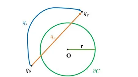
Fig.4.Safe velocity tracking and obstacle avoidance scenario.

According to the above statement,q˙d,q˙s, ande˙ were based on measurements of real positionqand velocityq˙, which did not require further consideration of the high-fidelity model.Therefore, it was referred to as a model-free controller.Of course, the model-based oneu=B−1(Dq¨s+Cq˙s+G−Ke˙) was also feasible for velocity tracking, which would performance better but was heavily dependent on the system model.Another idea of reducing model dependency is to regard the system parameters as a kind of disturbance.Denotingd≜Dq¨s+Cq˙s+GgivesBu=−Ke˙+d, where only matrixBis the system information and the other system parameters are not needed.Therefore, the importance is shifted to determining how to deal with the disturbance in system control problems, which will be discussed in Section IV.

Remark 7:The above discussions involve theoretical analysis or numerical experiments.In regards to the application of the robotic systems, there are some practical problems.For example, collecting sample data is not easy in real environments since the cost is high and the efficiency is low.To overcome its shortcomings, nowadays the training of robots is often carried out in a simulated environment (such as computer simulation), where a large number of training data can be obtained at a lower cost [58].Transfer learning is an effective approach to this topic, which indicates that the information or control strategy will be learned in a simulated environment and then transferred to real environment [59].As a subfield of transfer learning, sim-to-real mechanisms regard the control strategy of the robots as the transfer object [60].The real environment information usually includes the system dynamical model, which is complex.Local information,which is embedded in the sample data, helps to establish a relatively similar simulated environment.Although there are differences between the simulated environment and the real environment, a human’s prior cognition information such as the established physical equations and estimation of related parameters, could be considered in the simulation process.In this way, the simulated environment could be adjusted by later sample data to narrow the differences [61].After that, the agent learns interactively with the simulated environment and optimizes the control strategy, which is then transferred to the real strategy [62].All in all, the sim-to-real mechanism is a technical way to provide safety-critical control of the robotic systems, which deserves more investigation in the future.

IV.ROBUST QPS FOR UNCERTAIN NONLINEAR SYSTEMS

Given that there might be some random factors in the actual operating environment, it is necessary and significant to study uncertain control systems and robust QP formulation.This section will introduce three kinds of uncertainties, robust CLF-CBF-based QPs, ISS-CLF and ISSf-CBF, and corresponding potential approaches.

A.Uncertain Systems and Robust CLF-CBF-Based QP

Consider the following uncertain affine-control system:

whered(t,x) denotes the time-dependent and state-dependent external disturbance or system uncertainty with appropriate dimension.Writed(t,x) asdfor convenience.As we all know,the Lipschitz continuity offandgis a common assumption in the control problems, as is the disturbanced.

Assumption 1:The disturbanced(t,x) in (36) is Lipschitz continuous with respect to timetand statex.That is to say,there exist the positive constantsbx,btandb0such that for∀x1,x2∈Xand ∀t1,t2∈I(x0), there is

wherei=0,1,2,...,ais a positive constant, andτis the sampling time (the value ofτis usually related to the hardware condition which could be very small in practice).Under (43),the estimation error ofdis bounded as follows:

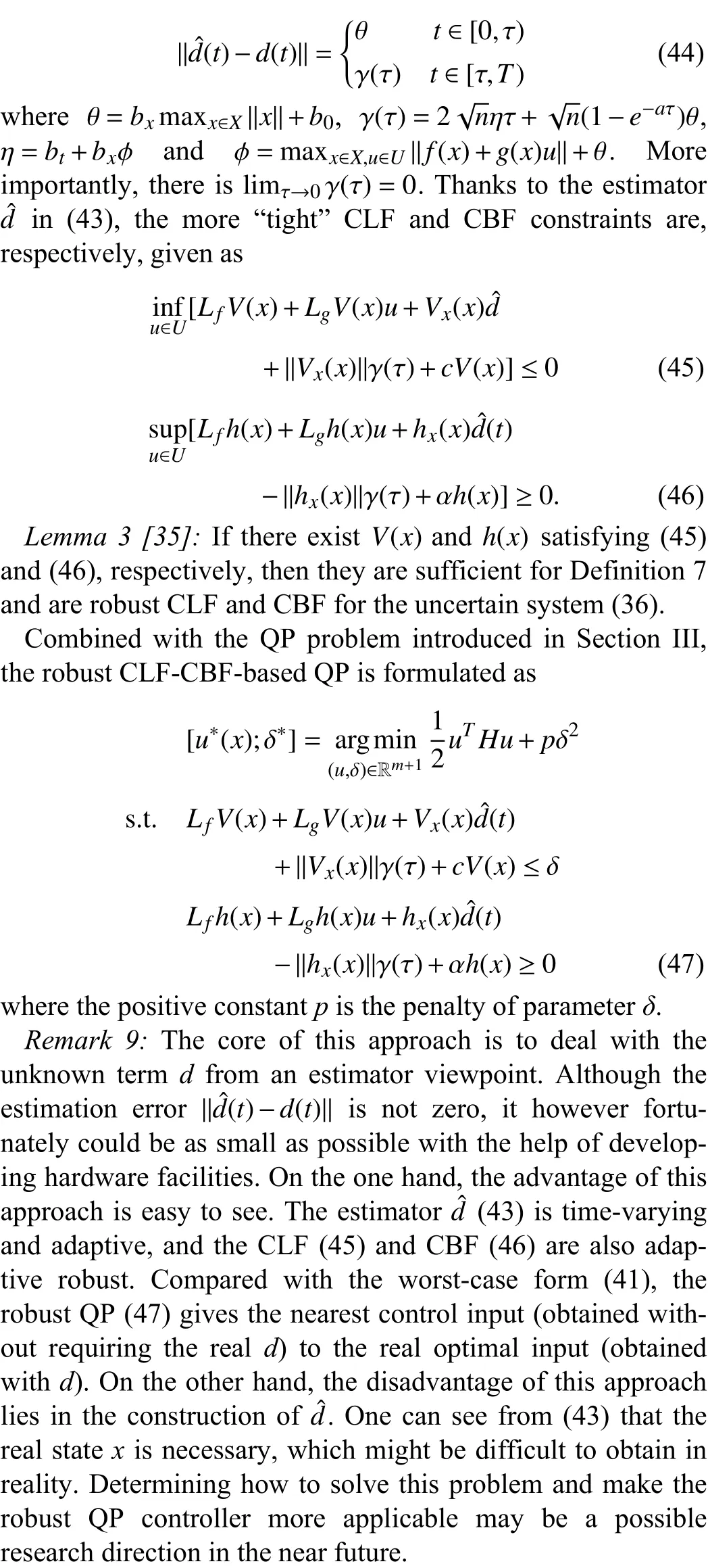
B.Uncertain Controllers and ISS, ISSf

This subsection will introduce another kind of uncertainty called input-to-state disturbance, which was discussed in [34].Compared with Section IV-A, the difference is that the disturbance is considered for controller.The control inputumight be affected by the time-dependent noise asu+d(t), whose dynamics is described as follows:

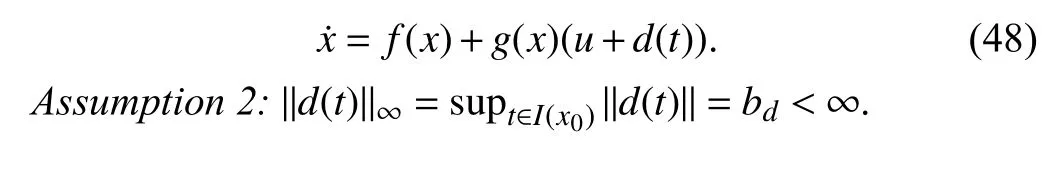
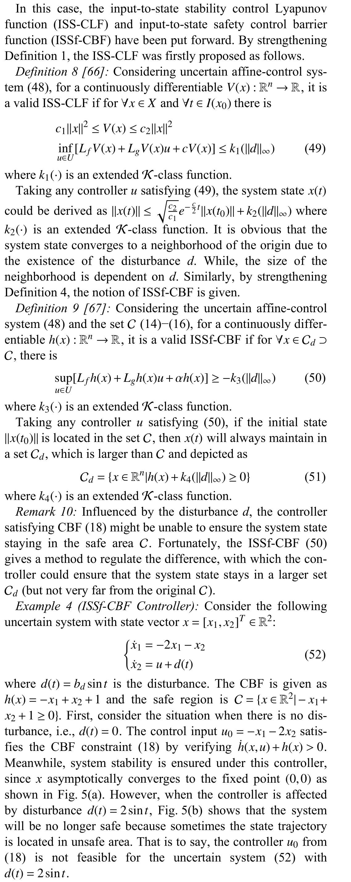
Fig.5.(a) The state trajectory under d(t)=0 and controller u0; (b) The state trajectory under d(t)=2sintand controller u0; (c) The state trajectory withd(t)=2sintand controller u.

Remark 12:The Assumptions 3 and 4 are so overly conservative, which need to be relaxed by other methods.Inspired by the data-driven approach in [69] and supervised regression method in [70], Tayloret al.constructed a learning framework for the termsaandbin [71].The robust QP problem was also studied by incorporating the learned information.However, the research on this topic is far from complete.Determining how to relax the assumptions and update CLFCBF-based QPs deserves more investigation in the future.In addition, the structure of the RL-CLF-CBF-based QP (57) is shown in Fig.6.

Remark 13:The Gaussian process (GP) could also be beneficial in estimatingf(x) andg(x) for the affine-control system(3), which is a popular way to describe the unknown terms[72].The uncertain model informationf(x) was considered with a distributionf(x)∼GP(m(x),k(x,x′)), wherem(x) was the mean function andk(x,x′) was the kernel function of the GP [73].Then, the GP-based CLF was proposed to attenuate the effects of uncertainties, and system stability was guaranteed with the maximal probability.In [74], the probabilistic bounds of model uncertainty were investigated, which were also used to rebuild CLF-CBF-based QP problems.Similar results for the discrete-time control systemxt+1=f(xt)+g(xt)u+d(xt) could be found in [75], whered(xt) was estimated with the Gaussian process.

Fig.6.A structure of the RL-CLF-CBF-based QP (57).

V.APPLICATIONS

This section will introduce some applications related to affine-control systems, such as mechanical systems, multiagent systems, adaptive cruise control (ACC) systems and lane keeping (LK) systems.The problem description of each part will be given and corresponding simulation experiments will be shown for easier reading.

A.QP in the Mechanical Systems

The mechanical systems are important in the physical world, whose dynamics are usually described as second-order nonlinear systems.For instance, in robotic systems, the system state may be related to position, velocity and acceleration,which need to be controlled at the force/torque level.It is common to see workspace constraints in mechanical systems since damage from the environment should be avoided.A robotic manipulator avoiding obstacles has been investigated based on a CBF control structure in [76], where multiple static and moving Cartesian position constraints were considered.Shaw-Cortezet al.used a robotic hand manipulated an unknown object and analyzed the semi-global practical asymptotic stability of the closed-loop system, which was also called as robotic grasping [77].In [78], a novel CBF was proposed to ensure constraint satisfaction of robotic grasping without slipping, which allowed to tune the velocity bounds to satisfy with the input constraint.

Besides obstacle avoidance and robotic grasping mentioned above, another physical scenario is the control of pendulums,including simple pendulum systems and inverted pendulum systems [79].The basic control objective is to keep the pendulum stable at some equilibrium point.The PD control method[80] and the feedback linearization strategy [81] have been frequently used to realize the stability of pendulum systems.According to the theoretical analysis in this survey, the CLFbased QP controller also works for this control objective.What is more, inspired by the safety constraint for the affinecontrol systems, the anti-swing control task could be achieved with the help of CBF control strategy, which motivates the following simulation experiment for the simple pendulum system.

Example 5 (CBF-QP-Based Safety Control for Second-Order Nonlinear Systems3The pendulum system model comes from [78].):As shown in Fig.7, consider a simple pendulum system whose dynamics is given by

Fig.7.The structure of a simple pendulum system.

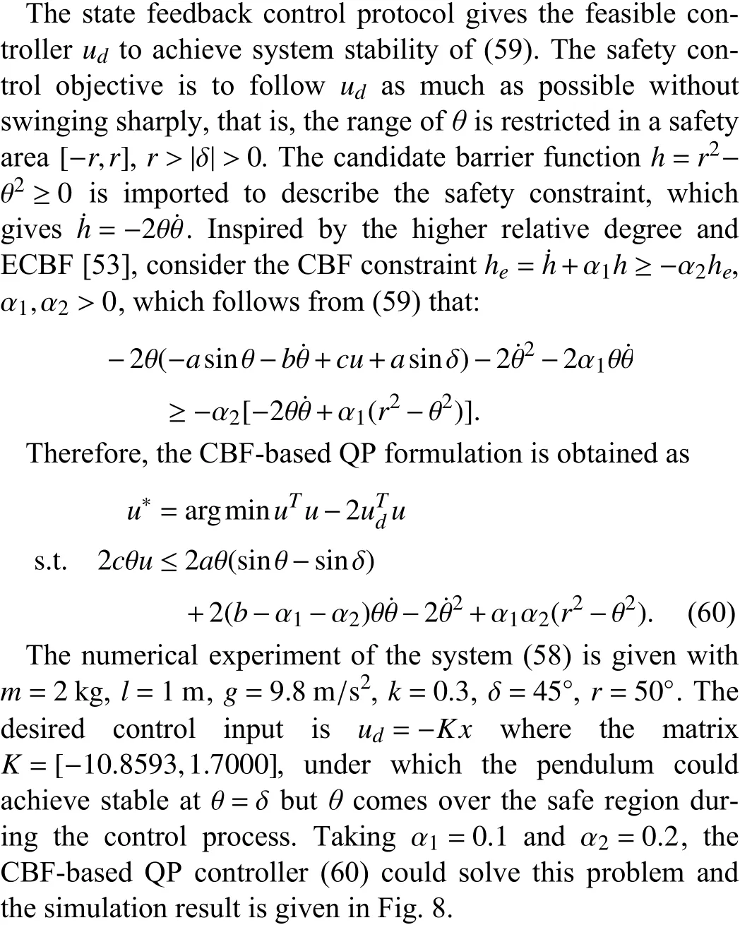
Fig.8.The trajectories of swing angle θunder different control inputs.The blue and orange lines represent the angle under control udand u∗, respectively.Both of them converge to 45°.The dotted line is the maximum bound of the swing angle.

B.QP in the Multi-Agent Systems

The MASs have been widely used in many fields, such as unmanned aerial vehicles, formation driving cars and so on.As important branches of the cooperative control of MASs,consensus control (stabilization and tracking) [82], [83], formation control (time-invariant and time-varying) [84], [85]and containment control problems [86] are increasingly interesting issues, which could be converted into the system stability control problems.

A common application of consensus control is the economic dispatch problem, which means that a team of generators provides electricity to a load or bus.The control objective is to obtain the amount of power provided by each generator while meeting the total amount requirement and minimizing the total costs [87].Distributed consensus-based algorithms have been applied to solve this problem [88], [89].More generally, another situation is the long duration autonomy problem, where a group of robots needs to charge with more than one battery [90].It is interesting to study the most effective way to make the system survive with the longest time, which has been modeled as a kind of CBF-based optimization problem [91]–[94].

Except for the consensus control mentioned above, the formation control of MASs was applied in the public transportation to optimize the allocation of transport resource in [95],where transportation efficiency was improved and the safety of the whole train group was ensured.The uncertain MASs were considered in [96], where the system dynamics was unknown and GP was used to learn the uncertainties.In addition, the distributed multi-robot task allocation and robust CBF have also caught much attention because of their potential applications in searching and monitoring, rescue and precision agriculture [97]–[100].In this section, an example about the cooperative control of MASs is provided as follows.

Example 6 (CLF-QP-Based Consensus Tracking Control of MASs4The system model comes from [83].):Consider the following general linear MAS:

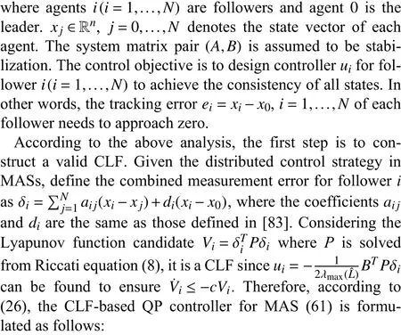
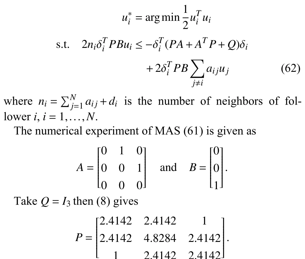
There are 4 followers and 1 leader in the whole system,whose communication topology is shown as Fig.9(a) containing a directed spanning tree.Fig.9(b) depicts the CLF-based QP controller solved from (62).Fig.10 shows the convergence of the errors, which indicates the achievement of consensus tracking and verifies the feasibility of the controller(62).

C.QP in the Adaptive Cruise Control Systems

Nowadays, there are worldwide challenges in the transportation and automotive field, such as the limited road capacity,driver errors, and so on [101].Adaptive cruise control (ACC)is worthy of attention due to its potential ability of contributing to these challenges [102].In an ACC system, a fleet of vehicles reaches a cruising speed (a kind of asymptotic stability), where the following vehicles should maintain safe following distance or time headway to the preceding vehicle (a kind of safety constraint) [103].

Fig.9.(a) The communication topology of the general linear MAS (61); (b)The CLF-based QP control inputs of all followers.

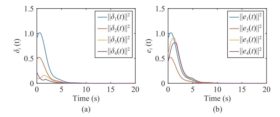
Fig.10.(a) The trajectories of the combined measurement errors δifor all followers; (b) The trajectories of the tracking errors eifor all followers.The initial states xi(0) are arbitrary vectors.In this simulation, they arex0(0)=[0.3433;0.1485;0.5752],x1(0)=[0.9586;0.6440;0.0486],x2(0)=[0.8403;0.4380;0.1741],x3(0)=[0.7626;0.7290;0.2798], andx4(0)=[0.6860;0.6970;0.4240].

The firstly introduced ACC in the market could be tracked back to the year of 1997, where a vehicle was driven at a preset speed by adjusting the throttle position [104].With the development of sensors, the second stage of ACC indicated that the vehicles could detect the vehicle ahead and adapt its own speed to maintain the pre-designed distance [105].In addition, thanks to the advent of vehicle-to-vehicle communications, more preceding vehicle information could be acquired by communication links, which allowed for smaller following distance and thus could increase the road capacity [106].Currently, cooperative ACC is under investigation and may greatly affect our lives in the future.

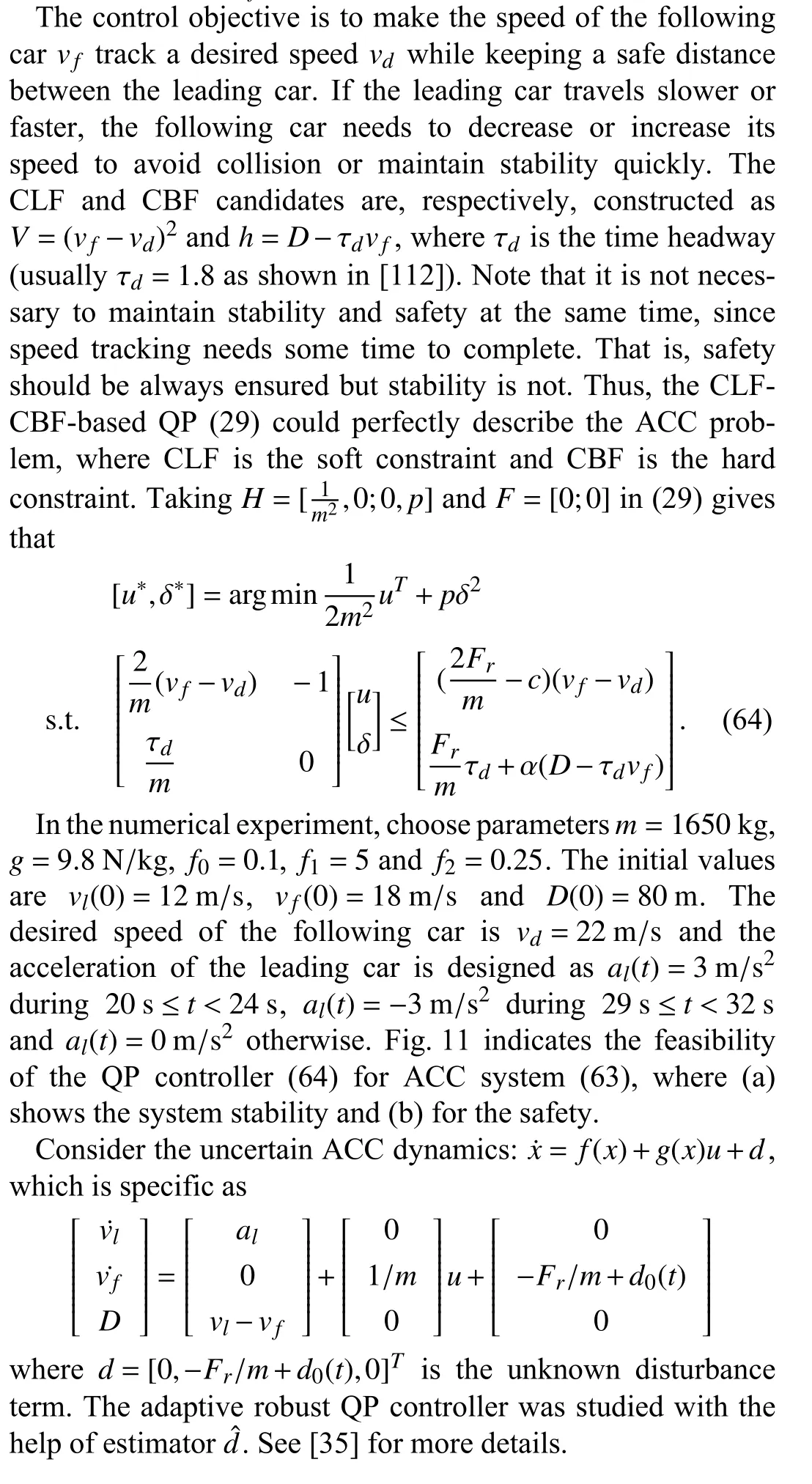
The commonly used control strategies, such as PID control,model predictive control and fuzzy logic control, have been applied in ACC problem [107]–[109].In addition, a QP control protocol was considered in [110], where both safety and performance as well as actuator limits were taken into account.Safety must be ensured which was seen as a hard constraint, and speed tracking was the soft constraint for the existence of QP solution in this problem.The following example illustrates the ACC model with vehicles moving in a straight line.

Example 7 (CLF-CBF-Based QP Control for ACC Systems5The system model and experimental parameters come from [35].):Consider a system composed by a leading car and a following one, whose dynamics is given as follows:

wherex=[vl,vf,D]Tis the state vector,vlandvfare, respectively, the speed of leading car and following car,Dis the following distance between two cars,alis the acceleration of the leading car,manduare the mass and controller of the following car, respectively [111].Fris the aerodynamic drag of the following car, which is modeled as the polynomial formFr=f0+f1vf+f2v2fwithf0,f1,f2as constant parameters.

D.QP in the Lane Keeping Systems

The lane keeping (LK) system plays an important role in the autonomous vehicle industry, where the car could automatically follow the anticipant lane.Different control strategies have been applied in automatic LK control such as the feedback control, adaptive control, yaw moment control, and so on[113]–[115].In [116], model predictive control method was imported and cast into the QP formulation for the LK system.Besides, the CBF also acts as a potential approach to deal with the LK problem given its safety requirement.Xuet al.proposed a CBF-based QP for safety and combined this with another performance-based controller (CLF or black-box legacy) [117].What is more, LK and ACC problems have been simultaneously realized based on the CLF-CBF-based QP controller, in which an experiment was developed on novel robot testbeds in a safe and inexpensive way [118].

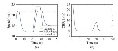
Fig.11.(a) The trajectories of the car speed; (b) CBF h=D−τdvf≥0.

The control objective of the LK problem is to keep the vehicle centered with curved lines under reasonable steering input,where its longitudinal speed is invariant and lateral speed is dynamically changing.To avoid driving off the road, the lateral displacement from the center of the laneyis required to be smaller than a boundymax, which is formulated as the constraint |y|≤ymax.In addition, the acceleration of the vehicle can not be too large considering the force limitamax, which is described as another constraint |y¨|≤amax.An example is given as follows to describe the feasibility of QP controller in the LK problem.

Example 8 (QP Control for Lane Keeping Problem6The system model and experimental parameters come from [32].):There are four variables in the LK problem, whose dynamics is

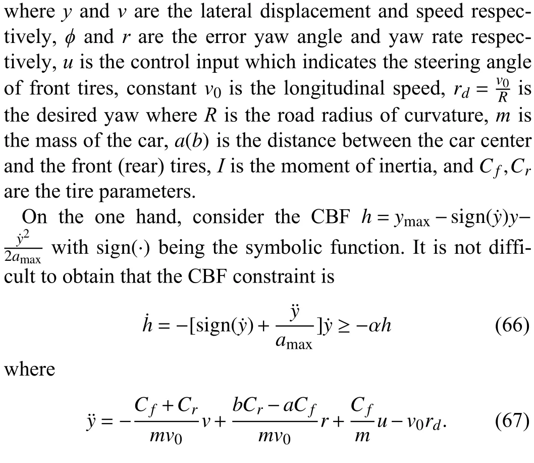
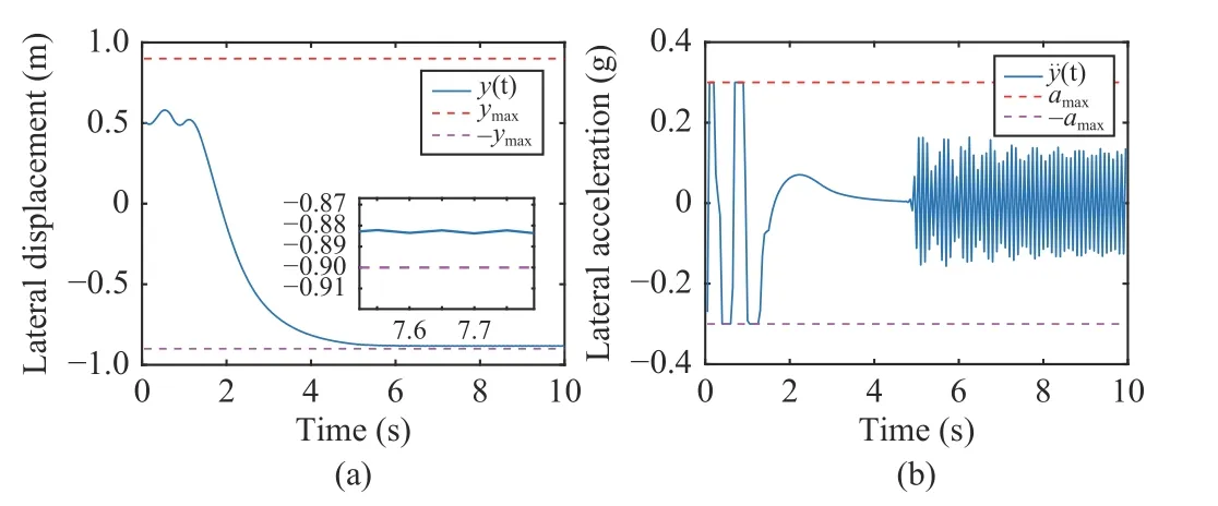
Fig.12.(a) The trajectory of the lateral displacement and its bounds; (b)The trajectory of the lateral acceleration and its bounds.Although there is oscillation in (b), the value of the amplitude is within the allowable range.

VI.CONCLUSION

In this paper, the CLF (ensuring the system stability) and CBF (ensuring the system safety) are combined with the QP optimization framework to obtain the optimal control protocol for nonlinear-affine control systems.Different forms of QP cost functions have been introduced and the robust CLFCBF-based QP has been reviewed for the uncertain systems.Afterwards, four kinds of applications have been given, where the recent literature results have been summarized and the corresponding examples describe the feasibility of QP optimization for nonlinear-affine control systems.Motivated by the above statements, there are some interesting and challenging topics that can be future research directions.Some of them are listed as follows.

A.Developing the Control Approaches for the Robotic Systems

Recently, the intelligent robot has caught worldwide attention, which is an important part of social development due to its wide uses in the fields of medical surgery, earthquake relief and industrial manufacturing [119].Considering that system safety is always required in its application, safety-critical control of the robotic systems is an essential and interesting topic.Nowadays, deep RL is widely used for the robot control problems such as the robot grasping [120] and walking [121],where the learning approach is based on a large number of data.Besides the above success, the deep RL also shows its capability of solving the challenging problems in the simulation robots such as the Atari [122], MuJoCo [123] and Star-Craft II [124].Nevertheless, sometimes the real environment could not offer infinite interactions to generate so much data,like in the real traffic control and autopilot.The sim-to-real mechanism is an effective method to deal with this problem.As introduced in Section III-B, it provides a technical way for robot training by transferring knowledge learned from the simulated platform to the real platform, in order to decrease the time and economic costs and to obtain more sample data easily [60].Under this mechanism, it is important to enhance the similarity of the simulated and real environments.Although the difference could be narrowed by later sample data in [61], it still remains an essential topic waiting to be studied.What is more, determining how to develop the transfer learning method for both simulated and real robots also deserves more investigation in the future.

B.Sketching the Safety Control for the Multi-Agent Systems

As we all know, safety is a basic requirement in robotic applications, which has inspired a lot of control methods in relevant works [125], [126].Besides, the Hamilton-Jacobi equation [127] and CBF [128] are also effective methods for the safety control objective such as obstacle avoidance, which however can not be used in high dimensional systems due to poor scalability.Meanwhile, safety is a hard constraint in the decentralized control framework because of the lack of the system information [129].Given the above concerns, Chen et al.studied the obstacle avoidance problem of MASs from a CBF viewpoint.The proposed controller was decentralized,supervisory, and applied in a general nonlinear robotic system with an arbitrary number of agents [130].The safe multi-agent interaction was investigated through the robust CBF in [75],where the heterogeneity of the agents in the real world could be regarded as the uncertainty.The robust CBF-based QP formulation was provided with a feasible controller, under which safety was always ensured during the agents' communication.One can see from the MASs field that system stability has been widely and deeply investigated with the help of Lyapunov theory.However, the situation is different for the system safety.As far as the authors' know, only some published literature consider safety in the cooperative control of MASs.One of the difficulties of safety control in the MASs is that it is necessary to avoid collision among multiple agents, which makes it harder to construct an appropriate CBF.Nevertheless, this topic is also a potential research direction from another perspective.

C.Designing the CLF and CBF for the Uncertain Systems

An important topic is to design a valid CLF or CBF without the requirement of the dynamical system models, which remains a challenging but significant problem since an accurate model is usually difficult to obtain in reality.An inaccurate model could describe affine-control systems with unknown items or system uncertainties, which deserves deeper investigations.Some learning approaches have been potentially imported in this issue in recent years.For example,Khan and Chatterjee proposed a novel Gaussian CBF for safety control in [131].As a flexible method to estimate any hyper parameters, GP was used to learn the kernel function to construct the CBF.In [132], Bayesian learning helped to gain a matrix variate Gaussian process distribution over system dynamics.More specifically, combined with an efficient covariance factorization, the aforementioned approach was used to learn the drift and input gain terms of a nonlinearaffine control system.Afterwards, the probabilistic CLF and CBF constraints were constructed and incorporated with the QP control policy, which could guarantee the stability and safety control of the uncertain systems.Despite all this, the control of uncertain systems is a persistent and ongoing topic,as the theoretical analysis is still weak.