
Application of shifted lattice model to 3D compressible lattice Boltzmann method
2023-10-11 07:55HaoYuHuang黄好雨KeJin金科KaiLi李凯andXiaoJingZheng郑晓静
Chinese Physics B 2023年9期
Hao-Yu Huang(黄好雨), Ke Jin(金科),4, Kai Li(李凯),4, and Xiao-Jing Zheng(郑晓静)
1School of Aerospace Science and Technology,Xidian University,Xi’an 710071,China
2School of Mechano-Electronic Engineering,Xidian University,Xi’an 710071,China
3Shaanxi Key Laboratory of Space Extreme Detection,Xi’an 710071,China
4Key Laboratory of Equipment Efficiency in Extreme Environment,Ministry of Education,Xi’an 710071,China
Keywords: lattice Boltzmann method,shifted lattice model,compressible flow,finite volume method
1.Introduction
Since the first paper about lattice Boltzmann method(LBM) appeared in 1988, the LBM[1–5]as a prominent tool in computational fluid dynamics has attracted much attention and become a major research hotspot.Unlike the traditional method based on macroscopic equations,the LBM is based on a mesoscopic kinetic model and obtains macroscopic quantities through statistics of distribution functions.The LBM is a multi-scale method, and its advantage is that the convection term is linear.Therefore, the LBM is applied to numerical calculation of various fluids, such as microscale flow,[6,7]turbulence,[8,9]multiphase flows,[10,11]blood flow,[12]and heat transfer.[13,14]
The research object of this paper is compressible fluid.Because the single distribution model adds new discrete velocity based on the isothermal model,and the specific-heat ratio is related to the spatial dimension of the model,it does not have real physical properties.While the double distribution function(DDF)model can adjust the specific-heat ratio and Prandtl number.So the double distribution function method[15–18]is adopted to construct a compressible fluid model.Of course,adding a distribution function will inevitably increase the amount of calculation.In 1998, Heet al.[15]first proposed the double-distribution model, which attracts wide attention because of its good stability and adjustable Prandtl number.Guoet al.[16]proposed a total energy distribution function to replace the internal energy distribution function.Liet al.[17]proposed a two-dimensional (2D) compressible finite difference DDF model and obtained satisfactory simulation results in high Mach number flows.Li and Zhong[18]proposed the potential energy distribution function model and applied the finite volume method to it.
Many researchers have made great efforts to develop three-dimensional (3D) compressible models.Kataoka and Tsutahara[19]proposed the D3Q15 model of compressible Euler equation, but this model only suitable for subsonic flows.Chenet al.[20]improved the Kataoka’s model and made the model suitable for higher speeds.Watari and Tsutahara[21]proposed the D3Q73 model,which can achieve a Mach number of 1.7.Liet al.[22]proposed the D3Q25 model of compressible Euler equation.According to Li’s model, Qiuet al.[23]introduced the total energy distribution function to optimize the D3Q25 model, and applied the Hermite expansion to the lattice Boltzmann model of D3Q27 to obtain a coupled double-distribution compressible model.
Although compressible model is being developed, the simulation of high Mach number flow is always problematic.In order to solve this problem,Huanget al.[24]proposed a discrete velocity model centered on the local flow velocity and the velocity varies with the local temperature.They successfully simulated shock tubes, and it is the first time that asymmetrical discrete velocity model has entered into people’s view.Sun[25,26]and Sun and Hsu[27]proposed an adaptive LB model in which the discrete velocity changes with local flow velocity and internal energy,thus the model can accomplish high-Mach simulation, but the relaxation time of their model must equal 1, which is a great limitation.Chopardet al.[28]and Hedjripouret al.[29]proposed one-dimensional (1D) asymmetric discrete velocity model: the model can successfully simulate a wide range of subcritical and supercritical flow, making it possible to practically use the asymmetric model.Frapolliet al.[30]proposed a novel shifted lattice model, adding another velocity to the original discrete velocity, so that the discrete velocity is no longer symmetric.They multiplied the equilibrium distribution function by a transformation matrix,and accomplished the conversion of the stationary coordinate system into the moving coordinate system,which greatly increases the calculation range of LBM.Saadatet al.[31]applied Frapolli’s shifted lattice model to D2Q9 and successfully simulated the supersonic shock compressible flow.But the disadvantage of transformation matrix is too complex and it is easy to generate a singular matrix, which is only suitable for a small discrete speed.
In the standard lattice Boltzmann equation (LBE), the discrete velocity of particles determines the type of computational grid.Generally, grids must be uniformly symmetric(regular hexagon, square).Although it is easy to construct such grids,they are not flexible enough to be applied to complex flow fields.In order to solve this problem,many scholars have conducted in-depth research on non-standard LBE models and proposed a variety of models.Reider and Sterling[32]first applied the fourth-order central difference scheme and the fourth-order Runge–Kuta scheme to LBM and proved the feasibility of the finite-difference LBM.Penget al.[33,34]proposed cell-vertex method, and they stored physical quantities on grid nodes and successfully used finite volume LBM to simulate the flow in a coaxial rotating cylinder.In this study,we use the third order monotone upwind scheme for scalar conservation laws(MUSCLs)finite volume scheme.
In this paper, we introduce the potential energy distribution function based on Li’s[22]D3Q25 density distribution function to create a new DDF model.In addition,a new shifted lattice model is proposed based on the linear equation.The 3D shifted lattice model is applied to the D3Q25 model to obtain better numerical stability.The rest of this article is organized as follows.In Section 2,we briefly introduce the DDF model,D3Q25 model and the shifted lattice model.In Section 3,we introduce the numerical method.In Section 4, we carry out numerical simulations of some typical compressible flows to prove the good effect of the shifted model.Finally, conclusions are drawn in Section 5.
2.The 3D compressible double distribution function model
2.1.Compressible D3Q25 LBM model
Li and Zhong[18]introduced the potential energy distribution function on the basis of the density distribution function, and proposed a DDF compressible LB model.An additional potential energy distribution function can be introduced to overcome the shortcomings of the Boltzmann Bhatnagar–Gross–Krook (BGK) equation that cannot present adjustable specific heat ratio nor Prandtl number.The functional model for this paper is the DDF LB model,and its dynamic equations are as follows:
whereZa=(ea-u)2/2,fαis the density distribution function,hαis the potential energy distribution function,andare the corresponding equilibrium distribution functions,eαis the discrete velocity of the particle,τfandτhare the relaxation time of density and potential energy respectively,τhfis the potential energy relaxation rate that can be determined from the following equation:
whenτf=τhthis model degenerates into the original BGK model,withτfdefined as
whereµis the viscosity andpthe pressure(p=ρRT), withRbeing the specific gas constant andTthe temperature.ThePrnumber can be created arbitrary by adjusting the two relaxation times as shown below:
Potential energy distribution function can be obtained easily from the following equation:
whereK=b-D,bis the number of degrees of freedom(DOFs),Dis the space dimension.
The D3Q25 based circular distribution function which is proposed by Liet al.[22]is shown in Fig.1.

Fig.1.Illustration of D3Q25 discrete velocity model.
2.2.The 3D shifted lattice model
In this study, we propose the shifted lattice model, by using a linear equation to replace the transformation matrix,thereby realizing the conversion of coordinates,increasing the feasibility of the model,and making the multi-discrete velocity model also able to use the shifted lattice model.Each discrete velocity is increased by a velocityvas shown in Fig.2.The magnitude of velocityvcan be a fixed value or change with the velocity of the flow field.In this work, we define that the value ofvis proportional to the sum of maximum and minimum velocity after each collision.Then we addvinto the initial symmetric discrete velocity to obtain a real discrete velocity
wherecαis the initial discrete velocity of Li’s D3Q25,[22]vnis the shifted speed obtained in then-th iteration,andis the real discrete velocity of then-th iteration.
The dynamic equation of the density distribution function is divided into the following two parts: flow process and coordinate transformation
We will adopt the MUSCL finite volume scheme to calculate Eqs.(9),(12),and(13).The specific content will be described in detail in the next section.

Fig.2.Illustration of shifted lattice model.
2.3.Boundary conditions
2.3.1.Non-slip wall boundary condition
Wall flow variables are as follows:
Under the non-slip wall boundary condition,non-equilibrium extrapolation scheme[35]is used.Density and potential energy distribution functions on the wall are expressed as
Equilibrium distribution functions are computed with the flow variables.The subscripts “cf” denotes the interface on the boundary and“in”denotes its neighbor cell.
At present,the shifted lattice model is suitable for isothermal wall conditions.While adiabatic wall conditions will produce some errors, and the results can be improved by multiplying the non-equilibrium term with a number less than 1.
2.3.2.Inlet flow boundary condition
where ∞denotes the inflow state.
2.3.3.Outflow flow boundary condition
3.Numerical methods
In order to capture the discontinuity well,we need to introduce artificial dissipation.There are two ways to introduce artificial dissipation.One is the model dissipation, and the other is the numerical dissipation from numerical methods.When the viscosity is very small, the model dissipation is unable to capture discontinuities without oscillation.So the numerical scheme is used to provide the additional dissipation.
Many researchers have applied different numerical schemes to LBM, such as, the weighted essentially technique[36]and the 6th-order compact finite difference method.[37]Although they are both high-resolution discretization schemes, they are more complex than the MUSCL scheme.[38–40]The MUSCL scheme is a simple spatial discretization scheme,which is very popular among researchers.
We have adopted the MUSCL finite volume scheme in the previous subsection.Taking the density distribution function for example,equation(1)can be rewritten as
whereΓis the corresponding grid boundary,Vis the volume of mesh,and ¯fαis the average distribution function on the grid,
withnbeing the normal vector in the outward direction, and¯Ωf,αthe average collision term.
It can be seen from Fig.3 thatn1ton6are the normal vectors of the six corresponding surfaces, with each surface having corresponding flux and area as follows:
whereΦα,i±1/2,j,k,Φα,i,j±1/2,k,andΦα,i,j,k±1/2are the numerical fluxes on each grid surface,the specific value is as follows:
whereandare the distribution function on the internal side and the external side of the interface (i+1/2,j,k).We use the third order monotonic upwind scheme for scalar conservation law with the smooth limiter to obtain the following values:
whereκ=1/3,ris the van Albada limiter[41]given by
withλbeing a small number, which is usually taken to be 10-12toavoid dividing by 0,and
Now, we can figure out the specific number of fluxΦ.Next,we use the sum of the product of the flux and the area of the six faces to simplify the integral in Eq.(20)into a linear summation formula,the dynamic equation can be obtained by simplification as follows:
The potential energy distribution function is treated in the same way as the density distribution function.

Fig.3.Numerical flux on grid surface.
4.Numerical simulations
A series of numerical simulations is conducted in this section to verify the stability and accuracy of the proposed compressible model,mainly simulating Riemann problems,Taylor vertex flow,Couette flow,Regular shock reflection,3D explosion in a box, and 3D flat-plate.In the simulation, the reference density isρref=1.0,the reference velocity isUref=1.0,and the reference temperature isTref=1.0.The characteristic temperatureTcis often a little bit higher than the maximum stagnation temperature in the whole flow field.
4.1.Riemann problems
Riemann problem is one of the core problems in computational fluid dynamics.In computational fluid dynamics, almost all high-precision schemes are based on solving Riemann problems.Owing to the Riemann problem including smooth solutions and discontinuous problems,it is a difficult and core problem of computational aerodynamics.
As a standard 1D problem, the length of shock tube is 1, the size of the calculate region isNx×Ny×Nz= 401×8×8.Both the exit and entrance are set as initial conditions, other boundary conditions are set as periodic boundaries.the specific-heat ratio isγ=1.4, the Prandtl number isPr=0.71,and the viscosity isµ=2×10⁻⁵.In this paper,two different examples are simulated, and the difference between the D3Q25 model with and without shifted lattice model is compared respectively.It is proved that the accuracy and stability of D3Q25 model can be improved by adding shifted lattice model.
The first example of the simulation is Sod shock tube,the initial conditions are as follows:
where the time step is Δt=1×10⁻⁵, and the characteristic temperature isTc=2.5.
Figure 4 shows the results of density, pressure, temperature,and velocity with shifted lattice model att=0.2 respectively.For a better comparison, the analytical solutions are also plotted.

Fig.4.Simulation results and analytical results from shifted lattice model of the Sod shock tube: (a)density,(b)pressure,(c)temperature,and(d)velocity.
The second example of the simulation is the stability contrast test,the initial conditions are as follows:
where the pressure on the left side is 1, the pressure on the right side is adjustable.We test the stability of the shifted lattice model by controlling the pressure ratio.The time step is Δt=1×10⁻⁵,and the characteristic temperature isTc=1,the size of the calculate region isNx×Ny×Nz=201×8×8.
Through testing, it is found that the maximum pressure ratio can reach 70 without adding the shifted lattice model.In the case of shifted lattice model, the maximum pressure ratio can reach 145.The simulation results are shown in Fig.5.When the pressure ratio is 75,the non-shifted model begins to oscillate and then diverges, while the shifted model has good stability.Obviously,the shifted lattice model can increase the stability of DDF model.

Fig.5.Speed comparison at pressure ratio 75.
4.2.Taylor vortex flow
This case is used to test the spatial accuracy of the present method.And this case has the following analytical solution:

Fig.6.Spatial accuracy validation of the present method.
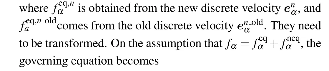
wherep0= 100.0,u0= 1.0,A=B= 2π,α=A2+B2,µ=0.001 is the shear viscosity,densityρ=2λ p,λ=0.005,time step is Δt=1×10⁻⁵,and the characteristic temperature isTc=144.The computational domain is set to be 0≤x ≤1 and 0≤y ≤1.The computation domain is discretized into 16×16×5,32×32×5,64×64×5,and 128×128×5.To test the order of the present method, the results from different meshes have been used to calculate L2 errors in velocity field.Figure 6 illustrates a model that is almost second-order accurate.Figure 7 shows the velocity profiles compared with analytical solutions at different times.It can be seen that the evolution is correct through the present method.
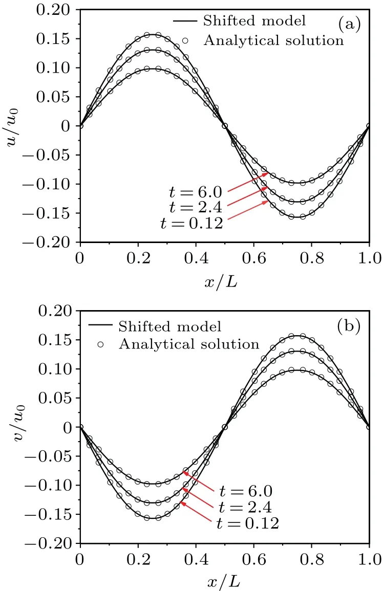
Fig.7.Comparison among velocity profiles of(a)u and(b)v at different times.
4.3.Couette flow
Couette flow is a classic test case driven by two parallel plates.For this problem, the computational domain has the initial conditions(ρ,T0,u,v,w)=(1,1,0,0,0).When simulation starts, the top plate moves at a constant velocityU0.In a steady state, the temperature profiles satisfy the following relation:
whereH=1 is the height of the two plates, andyis the distance of any point in the computation domain from the bottom plate.In the simulation, a meshNx×Ny×Nz=6×65×6 is used.The non-equilibrium extrapolation method is applied to the top and bottom wall, and periodic boundary condition is imposed on theyandzdirection.The viscosity isµ=8×10⁻³,and the time step is Δt=2×10⁻³.
The Prandtl numberPr=τf/τhis adjustable.The range of the Prandtl number is from 0.4 to 10 approximately.Figure 8 shows the temperature profiles compared with analytical solutions along theydirection forU0=1,b=5,andPr=1,3,5,8.It can be found that the simulation results and analytical results are in satisfactory agreement.

Fig.8.Temperature profiles along the y direction for different Prandtl numbers.
4.4.Regular shock reflection
A steady 2D compressible flow, i.e., a regular shock reflection on a wall, is considered in this test.This problem involves three flow regions separated by an oblique shock and its reflection from a wall.A shock wave of Mach number 2.9 is incident on the wall at an angle.The Dirichlet conditions are imposed on the left and top boundaries,respectively.
The bottom boundary condition is the reflection boundary, the right boundary is supersonic flow where the zerothorder extrapolation scheme is used.They-direction boundary is a periodic boundary,and the value of the entire flow field is set as the left boundary condition at the beginning.The size of the calculate region isNx×Ny×Nz=150×50×5.The time step is Δt=1×10⁻⁵,the characteristic temperature isTc=2,the viscosity isµ=1×10⁻⁵,the Prandtl number isPr=0.71.
Figure 9 shows the results of density, pressure, temperature,and velocity from the shifted lattice model: three distinct areas can be clearly seen in the picture, the incident angle is measured to be 29.05°[arctan(1/1.8)], of which the exact result is 29°.
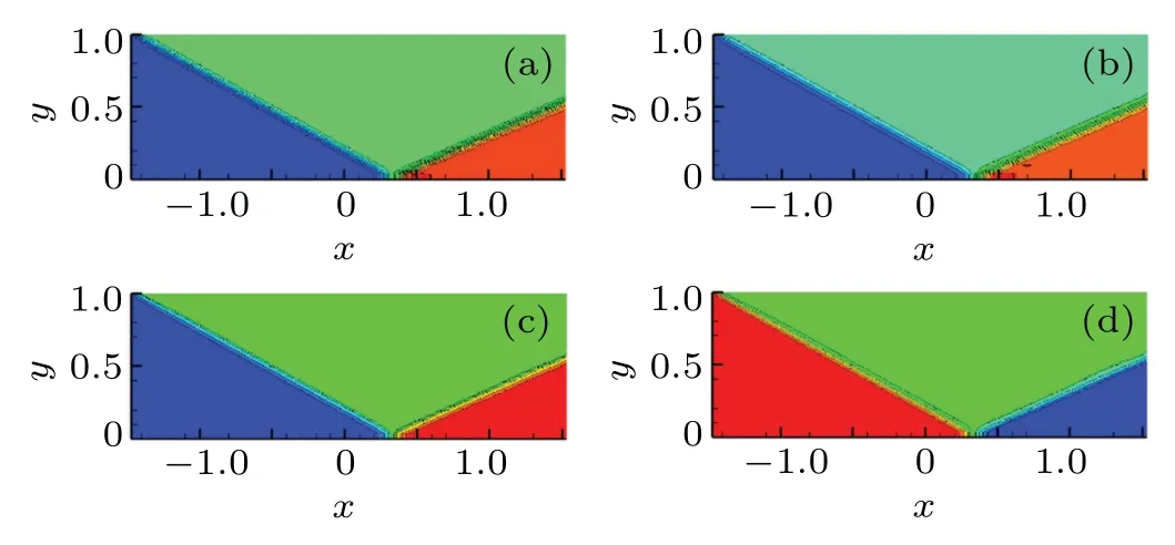
Fig.9.Simulation results of(a)density,(b)pressure,(c)temperature,and(d)velocity of regular shock reflection,obtained from shifted lattice model.
The residual curve of shifted model and non-shifted model for comparison are plotted in Fig.10.Because the distribution function is divided into two parts and the shifted lattice velocity changes with time,the convergence speed of the shifted model is slightly slower than that of the non-shifted model.The final residuals of both models satisfy the convergence condition.

Fig.10.Residual curves of regular shock reflection.
4.5.The 3D explosion in a box
In this subsection,we test the explosion in a box.[42]The results are shown in Fig.11.At the beginning of the simulation, the velocity in space is zero, the pressure and density in the sphere space are defined as follows:
Space sphere equation is defined as follows:
The dimension of space is[0,1]×[0,1]×[0,1],the size of the calculate region isNx×Ny×Nz=80×80×80,the time step is Δt=1×10⁻⁶, the viscosity isµ=1×10⁻⁵, the Prandtl number isPr=0.71,and the boundaries of these six surfaces are all periodic.

Fig.11.3D explosion in a box.
Figure 12 shows the density contour atz=0.4 andt=0.5,which accords well with results of Refs.[22,42].

Fig.12.Density contours for z=0.4,t=0.5: (a)simulation result of the present study and results cited from(b)Ref.[20]and(c)Ref.[36].
4.6.The 3D flat-plate boundary conditions
A 3D flat-plate(Fig.13)is simulated in this subsection to verify the feasibility of the shifted lattice model with a nonslip boundary.Previously,Carter[43]accomplished the numerical simulation of the 2D flat-plate supersonic boundary layer.With a 3D shifted lattice model added to the lattice Boltzmann method,the supersonic flat-plate boundary layer is simulated.Mach numberMa=3.0,Reynolds numberRe=1000,γ=1.4,Pr=0.72, the bottom boundary are used in a nonequilibrium extrapolation scheme,and both the front side and the back side are set as periodic boundaries.The size of the calculate region isNx×Ny×Nz=100×100×5.the time step is Δt=1×10⁻⁴.
Fig.13.3D flat-plate.
Figure 14 shows the distribution of flow field.

Fig.14.Flow field of flat-plate.
Figure 15 shows the ratio of the bottom pressure to the initial pressurePw/P0andu/u∞atx/L0=1 compared with Carter’s result,showing good agreement with each other.
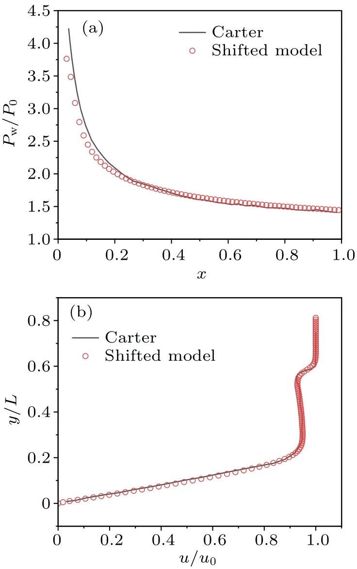
Fig.15.Comparison of (a) Pw/P0 versus x and (b) y/L versus u/u0 between Cater and shifted model for 3D flat-plate.
5.Conclusions
A D3Q25 LBM DDF compressible flow model and a shifted lattice model are established in this work.With the finite volume scheme, the shifted lattice model is applied to D3Q25 model, with numerical experiments including Sod shock tube, Taylor vortex flow, Couette flow, regular shock reflection, 3D explosion in a box, and 3D flat-plate.The numerical results obtained are basically consistent with the analytical solutions or simulation data in the existing literature,it is proved that the stability of D3Q25 DDF model can be improved by adding the shifted lattice model.This paper also has some shortcomings.Although the shifted model can increase the stability to a certain extent, the maximum Mach number of this model can only reach 3.In the future, the shifted model is hoped to combine with multiple-relaxationtime LBM to simulate higher Mach number.Overall,this work further optimizes the 3D compressible model,and has guiding significance for the simulation of high Mach supersonic flow.
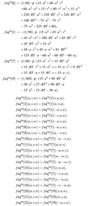
Appendix A: Discrete equilibrium distribution function of 3D LB model
Acknowledgements
We sincerely thank Dr.Pan Dong-Xing for his help with the mesoscopic method.
Project supported by the Youth Program of the National Natural Science Foundation of China (Grant Nos.11972272,12072246, and 12202331), the National Key Project, China(Grant No.GJXM92579), and the Natural Science Basic Research Program of Shaanxi Province, China (Program No.2022JQ-028).
猜你喜欢
Chinese Physics B(2023年2期)2023-03-13
Chinese Physics B(2023年1期)2023-02-20
机械研究与应用(2022年4期)2022-09-15
机械研究与应用(2022年3期)2022-07-25
火花(2022年4期)2022-06-16
现代装饰(2021年2期)2021-07-21
知识经济·中国直销(2017年12期)2018-01-03
知识经济·中国直销(2017年6期)2017-06-13
时代文学·上半月(2015年9期)2015-12-21

- Chinese Physics B的其它文章
- Dynamic responses of an energy harvesting system based on piezoelectric and electromagnetic mechanisms under colored noise
- Intervention against information diffusion in static and temporal coupling networks
- Turing pattern selection for a plant–wrack model with cross-diffusion
- Quantum correlation enhanced bound of the information exclusion principle
- Floquet dynamical quantum phase transitions in transverse XY spin chains under periodic kickings
- Generalized uncertainty principle from long-range kernel effects:The case of the Hawking black hole temperature