
Optimal zero-crossing group selection method of the absolute gravimeter based on improved auto-regressive moving average model
2023-12-02 09:22ZongleiMou牟宗磊XiaoHan韩笑andRuoHu胡若
Chinese Physics B 2023年11期
Zonglei Mou(牟宗磊), Xiao Han(韩笑), and Ruo Hu(胡若)
1College of Electrical Engineering and Automation,Shandong University of Science and Technology,Qingdao 266590,China
2National Institute of Metrology China,Beijing 100029,China
Keywords: absolute gravimeter,laser interference fringe,Fourier series fitting,honey badger algorithm,multiplicative auto-regressive moving average(MARMA)model
1.Introduction
The precise measurement of gravitational acceleration is of great significance in the fields of metrology, geophysics,and geodesy.[1–4]During the operation of a laser interferometric absolute gravimeter, the free-fall mirror and the reference mirror in the Michelson interferometer interfere with each other under light reflection.Laser interference fringes can be obtained.The free-fall time and trajectory are calculated through the laser interference fringes.Finally,the value of gravitational acceleration is obtained by the least-squares method.At present, there are three methods for processing the laser interference fringes of absolute gravimeters: twosample zero-crossing detection method, windowed seconddifference method, and complex heterodyne demodulation method.The two-sample zero-crossing detection method calculates the zero-crossing point by interpolating the two sample points that are closest to the zero point and have opposite signs.The windowed second-difference method with an added window is to set a time window of a certain size and set a threshold value according to the peak and valley values within the time window.When the sample points within the threshold range selected by the threshold value are close to a straight line,a straight line is fitted to calculate the zero-crossing point.The complex heterodyne demodulation method is performed to iteratively outline a suitable signal on the sampled swept signal, narrowing its frequency band to a position close to the zero frequency.The final gravitational acceleration is obtained by nonlinear fitting.Svilov compared the differences of these three methods with the same absolute gravimeter.[5]The two-sample zero-crossing detection method has high requirements on computer performance and relatively poor accuracy,but it is widely used due to its simple calculation rules.The windowed second-difference method is slower in the process of finding the zero-crossing points of fitted line.The complex heterodyne demodulation method is suitable for seriously under-sampled signals and requires prior knowledge of the signals.
It is not necessary to fit all time–displacement data for gravitational acceleration calculation.A zero crossing is taken at everyNcrossing point,and the subsequent least-squares fitting is performed.Zumberge used the JILA absolute gravimeter to measure the acceleration of gravity over a falling distance of 17 cm.[6]The number of zero-crossing groups for each drop is 150.Least-squares fitting was performed on 45 entries of time–displacement data obtained by the twosample zero-crossing detection method.The resulting gravitational acceleration has a standard deviation of 6–10 µGal.Niebauer obtained the interference fringes from the data acquisition module of the absolute gravimeter of FG5.[2,7–9]The two-sample zero-crossing detection method was then used to calculate the zero-crossing points based on the interference fringe data.The number of zero-crossing groups for each drop was 700.The standard deviation of calculated gravitational acceleration was 5–8 µGal.Wu calculated the zerocrossing points and the falling distance by improving the twosample zero-crossing detection method.[10,11]The number of zero-crossing groups for each drop was 400.The gravitational acceleration obtained from the experimental prototype can be measured within the standard deviation of 10 µGal.Feng simulated the NIM-3A absolute gravimeter effect under self-vibration conditions.[12]The number of groups of time–displacement data calculated by the zero-crossing method was set to 700.Finally, the least-squares fitting method was used to obtain the gravitational acceleration value.The average deviation of the fitted gravitational acceleration from the preset gravitational acceleration was within 1.8µGal.The larger deviations reach 367.6 µGal and 26.2 µGal when the residual amplitudes are 5 nm and 0.3 nm, respectively.Nowadays,most researchers select a fixed number of zero-crossing groupsNfor least-squares fitting.The sampling rate is fixed throughout the drop.However, the frequency of laser interference fringe gradually increases with time.The data are sparse in the early stage and dense in the late stage, which will have a certain impact on data fitting.[13]
In this paper,the Fourier series fitting method is proposed to find the zero-crossing points.The time interval of the falling process is divided into five segments.The number of optimal zero-crossing groups in each section is calculated, and then least-squares fitting is carried out.Finally, the mean value of the gravitational acceleration in each segment is obtained.The method of Fourier series fitting can reduce the fitted residual and improve the accuracy of estimated gravity.With the increase of the laser interference fringe frequency, the number of optimal zero-crossing groups will also change.The error between the obtained gravitational acceleration and the reference value is further reduced to improve the fitting accuracy.
2.Methods
2.1.Working principle of absolute gravimeters
The working principle of laser interferometric absolute gravimeters is shown in Fig.1.A laser beam emitted by the laser is divided into two beams through the beam splitter: vertical upward and horizontal rightward.These two kinds of laser beams interfere after the reflection of the free-fall mirror and the reference mirror.An interference signal is received by the photodetector.The time–voltage data (ti,Ui) are obtained by the digital acquisition module.The falling process is carried out in a vacuum environment.Therefore,the falling mirror is only subject to the action of gravity.The frequency of interference fringes increases with time as the falling speed becomes increasingly faster.The ideal laser interference fringe is shown in Fig.2.[14–16]
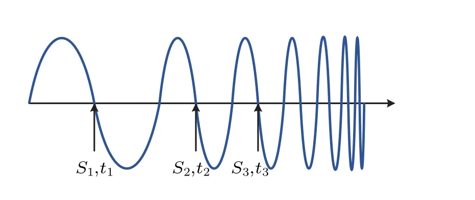
Fig.2.Ideal laser interference fringe.
2.2.Principle of time–displacement data calculation
The basic principle of Fourier series fitting is to process the data points obtained by the data acquisition module and multiply the voltage values of two adjacent data points.If the condition ofUi×Ui+1≤0 is satisfied, there must be a zerocrossing pointt0in the period oftitoti+1.It is known that the zero-crossing point is within the range of [ti,ti+1].Based on the results of previous experiments, the first 200 points oftiand the last 200 points ofti+1must be selected for Fourier series fitting.The Fourier series expansion is shown below:
where the fitted equationf(t)=0.We then calculate the exact zero-crossing point in the [ti,ti+1] interval by fixing the zero-crossing point range and then performing a Fourier series fitting.The calculation time for the Fourier series fitting is shortened, while the calculation accuracy of the zerocrossing point is improved.According to the working principle of the Michelson interferometer,the difference between the two interferometric beams varies by a quarter of the laser wavelength,which produces a zero-crossing point.The falling distance is linearly related to the zero-crossing pointtktime.The distanceSkthat dropped at momentkis calculated according to
whereλis the laser wavelength, andkis the zero-crossing times.The principle of the Fourier series fitting is shown in Fig.3.
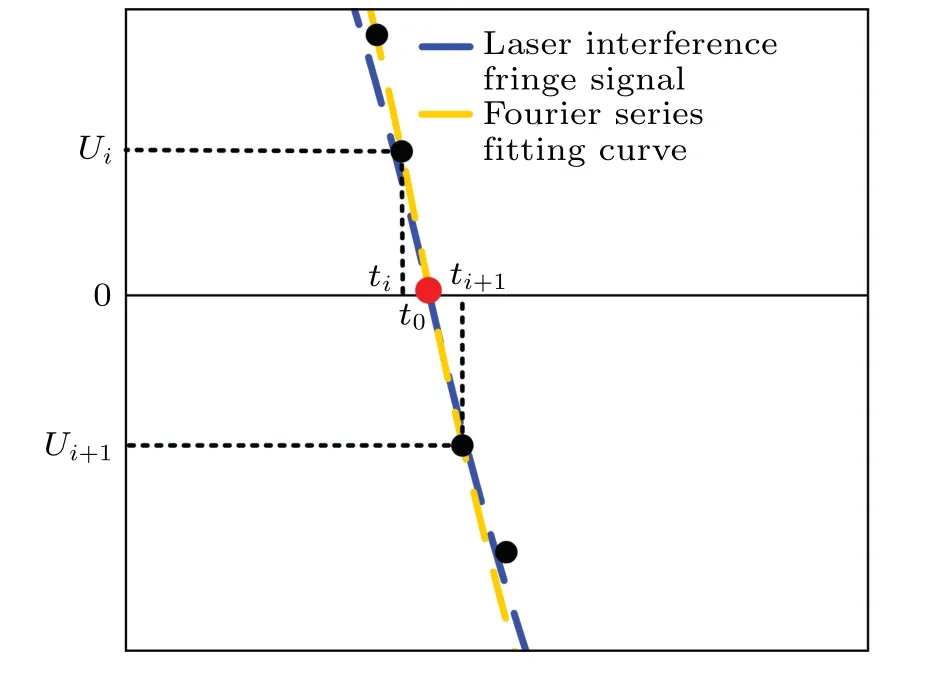
Fig.3.Principle of the Fourier series fitting.
3.Multiplicative auto-regressive moving average model construction and optimal zerocrossing group prediction
3.1.Calculation of instantaneous frequency of the laser interference fringe signal
When the frequency of a laser interference fringe signal increases linearly with the drops, this signal is called linear modulated signal.[17,18]To find out the instantaneous frequency of the laser interference fringe signal,the signal is subjected to Hilbert transformation,[19]as shown below:
where ˜U(t) is the convolution of the original laser interference fringe signalU(t), and the impulse response functionh(t)=1/(πt).The analytical signalz(t)of the original laser interference fringe signalU(t)is
Based on the analytical signal,its instantaneous phase can be calculated as follows:
The phase of the analytical signal differs from the original signal byπ/2.Its positive frequency produces a shift of-π/2,and its negative frequency produces a shift ofπ/2.To find the instantaneous phase of the original laser interference fringe signal,the following equation is used:
The instantaneous frequency of the original laser interference fringe signal is calculated from the phase derived from Eq.(6).Thus, the frequency of the laser interference fringe signal is calculated using
wheref0is the initial frequency, andkis the changing rate of the signal frequency.If it is necessary to obtain a fixed frequency band in the laser interference fringe signal,the corresponding time period can be determined using Eq.(7).
3.2.Honey badger algorithm to acquire datasets
The honey badger algorithm[20,21]is used to find the optimal solution in the solution space and to calculate the number of optimal zero-crossing groups for a fixed frequency band.We first initialize the number and location of the honey badger population,as shown below:
wherelbiis the minimum value of the number of zero-crossing groups,ubiis the maximum value of the number of zerocrossing groups, andr1is a random number between 0 and 1.Based on the concentration of prey and the distance between the honey badger and the prey,the movement speed of the honey badger is determined by the intensity of smell.The smell intensity of the dense badger is shown below:
wherer2is a random number between 0 and 1,Sis the prey concentration intensity,anddirepresents the distance between the prey and the current honey badger individual.
We define and update the density factor according to the number of iterations,as shown in below:
whereCis a constant greater than 1 (the default value is 2),andtmaxis the maximum number of iterations.
By calculating the density factor,the new position of the individual honey badger is updated according to whether the random number is less than 0.5.If the random number is less than 0.5, the honey badger position is updated by Eq.(11).Otherwise,the honey badger position is updated by Eq.(12).
wherer3,r4,r5,r6,andr7are random numbers between 0 and 1;βrepresents the honey badger’s ability to obtain prey(with a default value of 6);xpreyis the location of the prey;andxnewis the new location of the honey badger.Fis primarily used to change the search direction and prevent the honey badger from getting stuck into a local optimum.
The population fitness is calculated based on the new position of the continuously iterated honey badger population.Thus, the global number of optimal zero-crossing groups for the entire population is obtained.If the number of iterations does not meet the termination condition, the number of honey badger individuals,the global number of optimal zerocrossing groups, and the minimum fitness are updated until the condition is satisfied.Because the honey badger algorithm takes a long time to calculate the optimal number of zerocrossing points,it is necessary to build a mathematical model to adapt to the actual working conditions.
3.3.Prediction model multiplicative auto-regressive moving average for the number of optimal zero-crossing groups
The autoregressive moving average (ARMA) model is used to predict the subsequently generated data by the pattern of the previous data.The time seriesxsatisfies
wherextis the number of optimal zero-crossing groups in thetfrequency band, [φ1,φ2,...,φp] is the autoregressive coefficient,εtis the independent and identically distributed random variable series,and[θ1,θ2,,...,θp]is the moving average coefficient.In addition,the appropriate model is determined by autocorrelation function (ACF) and partial correlation function(PACF).If both ACF and PACF are trailing,the time series ofxis considered to obey the ARMA(p,q)model.[22]
The number of optimal zero-crossing groups obtained by the honey badger algorithm is used as the dataset for the ARMA model.Because the difference in the number of optimal zero-crossing groups in different frequency bands is small,the ARMA model is selected for training, which shows that the data change trend is not obvious.Therefore, the data of the training model are multiplied to feature a large amplitude change trend.Thus,the multiplicative autoregressive moving average (MARMA) model is constructed.The Akaike information criterion(AIC)as a measure of good or bad statistical model fit is defined[22]as
wherekis the number of parameters to be estimated in the model,andLis the likelihood function.To determine the optimal order of MARMA, the value of the number of optimal zero-crossing groups is substituted to calculate the AIC to filter the most suitable order.The specific prediction model is obtained by parameter estimation with known models and orders.Finally,the number of optimal zero-crossing groups for each frequency band is predicted based on this model.
4.Experimental results and analysis
4.1.Test platform
The NIM-3C gravimeter is an absolute gravimeter developed independently by the National Institute of Metrology of China.It uses a laser as the light source and converts the optical signal into an electrical signal.The laser interference fringe signal is further processed.The fall time is obtained from the clock signal synchronized by the atomic clock.The NIM-3C absolute gravimeter is placed in the base gravity experiment building comparison hall for testing by the National Institute of Metrology, Changping campus.The absolute gravimeter hardware experimental platform is shown in Fig.4,in which an ion pump is used to pump out the air in the vacuum chamber.The vacuum chamber is used to provide an environment for the falling object.The interferometer is used to acquire laser interference fringes.The vibration sensor is used to collect the vibration signals of the absolute gravimeter.The supporting platform and supporting legs are used to support the vacuum cavity,ion pump,and other equipment that do not come into direct contact with the interferometer.

Fig.4.Absolute gravimeter hardware experimental platform.
4.2.Calculation of time–displacement data
The total acquisition time of each drop is 0.25 s,of which 0.06–0.16 s is the time of free fall.The data of time period of free fall are then processed as follows.First, the voltages measured during the free fall are multiplied by 2.The data that satisfyUi×Ui+1≤0 are then used to construct two new voltage data matricesX1andX2and two new time matricest1andt2, whereX1andt1are the data points on the left side of zero crossing andX2andt2are the data points on the right side.The number of zero-crossing groups is set to 700.According to the position of the original data matrix int2,the first 200 points and the last 200 points int2(i) are selected as the time window.The data are substituted into Eq.(1)for a threeorder Fourier series fitting.Then,fi(x) corresponding to the zero-crossing point is obtained.
In the same time window, the zero-crossing point is calculated by the windowed second-difference method[5].The peak-valley value of the signal is 2A, and the threshold value is set asKso that the sampling points in[-KA,KA]approach a straight line.The sampling points in this interval are fitted linearly to find the zero-crossing point.The fitted residuals of the two zero-crossing points in the 100th time window are compared in the free-fall time period.The Fourier series fitting and the windowed second-difference method are compared,as shown in Fig.5.The comparison of fitted residuals of the two methods is shown in Table 1.
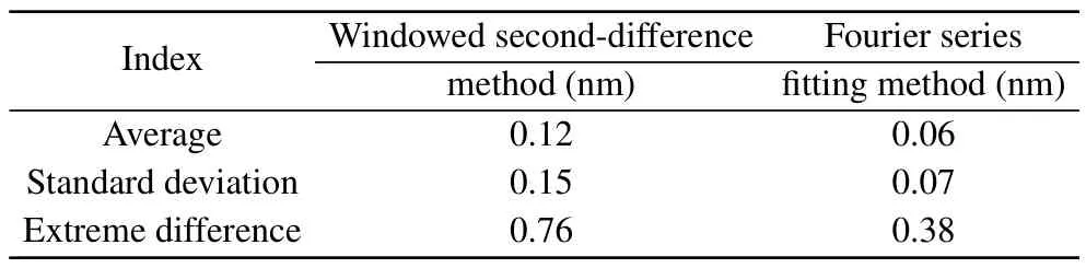
Table 1.Comparison of residuals fitted by the two different zerocrossing methods.
As shown in Fig.5,the residuals of the Fourier series fitting are within±0.2 nm.The fitted residuals of the windowed second-difference method are within±0.4 nm.In terms of the fitted residuals of the zero-crossing algorithm,the Fourier series fitting method is more concentrated around zero, with smaller standard deviation and more concentrated residual error.Therefore,this method is closer to the measured value and more stable than the windowed second-difference method.
While the two-sample zero-crossing detection method is used to interpolate the data points to the left and right of the zero-crossing point, the improved two-sample zero-crossing detection method is used to set a noise ceiling threshold to get the data that satisfy the condition ofUi×Ui+1≤0.The data points to the left and right of the zero-crossing point are then analyzed separately to determine whether there are sampling points between them, and the corresponding formula is used to calculate the result.The corresponding zero-crossing points are obtained using the two-sample zero-crossing detection,[5]improved two-sample zero-crossing detection,[10]and Fourier series fitting methods.From Eq.(2), the falling distance corresponding to the zero-crossing point is found, and thus the gravitational accelerationgis calculated.Ten groups of laser interference fringes are selected for calculation.The gravitational accelerationg0standardized by the National Institute of Metrology, Changping campus, is used as the reference true value in this paper.The error between the gravitational accelerationgand the reference valueg0of the three zero-crossing methods is calculated.The Fourier series fitting method improves the measurement accuracy compared with the two other zero-crossing methods.The improvement percentage in accuracy is shown in Table 2.
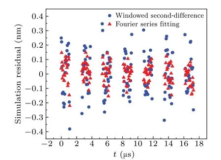
Fig.5.Comparison of fitted residuals between the two methods.
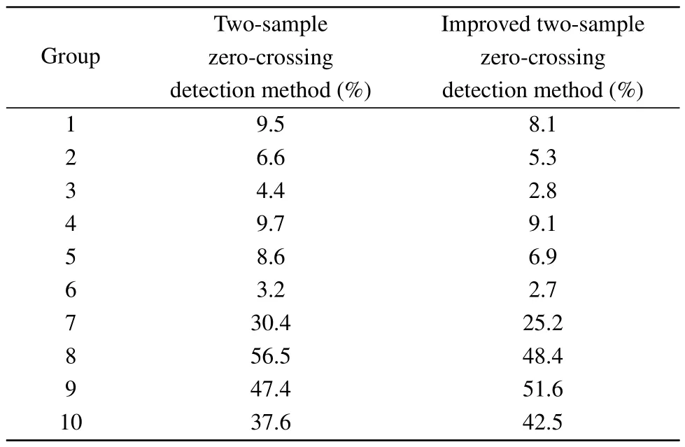
Table 2.Accuracy improvement percentage of method 1 and method 2.
As shown in the comparison of the 10 data groups in Table 2,the accuracy of the gravitational acceleration calculated by the Fourier series fitting method is improved by 20.6%on average compared to the two-sample zero-crossing detection method.The average improvement in accuracy compared to the improved two-sample zero-crossing detection method is 14.1%.Therefore,the Fourier series fitting method is superior in calculating the zero-crossing points of the drop.
4.3.Construction of the optimal zero-crossing group number dataset
Through the selected laser interference fringe data, the distance of the falling process can be calculated.The fall time is divided into five equal intervals to calculate the zerocrossing points based on the Fourier series fitting method.The time difference ∆tand the drop distance of ∆hare obtained.The formula for the gravitational acceleration is
where ∆tiis the time difference,∆hiis the falling distance corresponding to ∆ti,vis the falling velocity, andgis the acceleration of gravity.In the equation,the falling velocity and the gravitational acceleration are unknown.Therefore,at least two sets of data are needed to find the acceleration of gravity.The simultaneous calculation equation of two adjacent sets of data is given as
The gravitational accelerationgican be obtained,andg0is the reference value.The honey badger population size is initialized.Assume that the population consists of 100 honey badger individuals, each of which is a one-dimensional variable.The objective function of the honey badger algorithm is set to be the sum of the absolute values of the differences betweengiandg0,as shown below:
According to Eq.(18),by calculating and comparing the fitness of each honey badger individual, the global optimal solution is obtained, which is the number of optimal zerocrossing groups in the time period.The laser interference fringe signal is transformed by the Hilbert transformation.According to the instantaneous phase of the analytical signal,the instantaneous phase and frequency of the original signal can be calculated.The signal is divided into five segments at equal time intervals.The instantaneous frequency range of each segment can be calculated according to the obtained frequency expression off=f0+kt.The number of optimal zero-crossing groups is set for each of the five segments.The zero crossing and falling distance of each frequency band is then calculated according to the number of optimal zero-crossing groups.The generated time–displacement data are subjected to leastsquares fitting to calculate the gravitational accelerationgiof the frequency band.Finally, the mean valueis calculated using
wheregiis the gravitational acceleration calculated for a single frequency band, andis the final gravitational acceleration value.Seven groups of laser interference fringe data are selected.The number of optimal zero-crossing groups of the five parts in each group of data is calculated,as shown in Table 3.The convergence process of the first set of data according to the honey badger algorithm iteratively searching for the optimal zero crossing is shown in Fig.6.
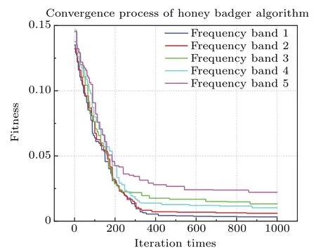
Fig.6.Convergence process of the honey badger algorithm.
4.4.Prediction of the optimal number of zero-crossing groups based on the MARMA model
The number of optimal zero-crossing groups is used as sequence data to build the model.The number of optimal zero-crossing groups is then predicted to calculate the gravitational acceleration of the absolute gravimeter.There are seven groups of data in the dataset.The first four groups of data in Table 3 are taken as the training set and data of groups 5–7 as the testing set.Because of the small difference of the objects involved in model fitting, the first four sets of data are first multiplied to amplify the change pattern.The model type is confirmed by the tailing off or truncation of the ACF and PACF.The ACF of the number of optimal zero-crossing groups is shown in Fig.7.The PACF of the number of optimal zero-crossing groups is shown in Fig.8.
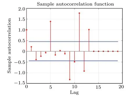
Fig.8.Partial correlation function of the number of optimal zerocrossing groups.

Table 4.AIC values of each order model.
As shown in Figs.7 and 8, the ACF and PACF are both trailing.Therefore,the MARMA model is used to predict the number of optimal zero-crossing groups.The AIC values are calculated to determine the order of the model.The AIC values for each order of the model were compared, which are shown in Table 4.
The model with the smallest AIC is selected to ensure a simple structure and accuracy.As shown in Table 4, the AIC is calculated for the training with the number of optimal zerocrossing groups.Whenp=2,q=2, the AIC is minimum.In turn, the MARMA (2, 2) model is fitted.The number of optimal zero-crossing groups in the test is calculated by the prediction model in the following equation:
The number of optimal zero-crossing groups is predicted according to the model.The MARMA (2, 2) model predicts the results of the number sequence,as shown in Fig.9.
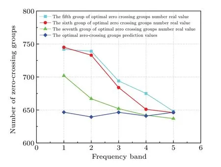
Fig.9.Results of the MARMA(2,2)model prediction.
As can be seen from Fig.9,for the model established by the training set, the relative errors in predicting the number of optimal zero-crossing groups from group 3 to group 7 are 0.066, 0.076, and 0.029, respectively.The number of optimal zero-crossing groups calculated by the MARMA model is used to extract the corresponding time–displacement data.The obtained data are fitted by Fourier series, and finally, the gravitational accelerationgis obtained.The accuracy of the two methods listed in Table 5 is improved by different percentages compared with the fixed zero-crossing groups using the two-sample zero-crossing detection method.
In Table 5,method 1 is the number of fixed zero-crossing groups,which is 700,and method 2 is the number of optimal zero-crossing groups,both by Fourier series fitting.As shown in Table 5, method 1 and method 2 have different degrees of improvement compared to the fixed zero-crossing groups by the two-sample zero-crossing detection method.[5]The accuracy of method 2 is improved by more than 25% compared to method 1 on average.The falling process is divided into five frequency bands.The number of optimal zero-crossing groups for each band is calculated by the honey badger algorithm.The first four groups of data are trained in the MARMA model to predict the optimal number of zero-crossing groups in each frequency band.According to the last three groups of laser interference fringe data, the number of optimal zerocrossing groups and the fixed number of zero-crossing groups are used for calculation.It is shown that the optimal number of zero-crossing group method in this paper effectively improves the accuracy of gravity.
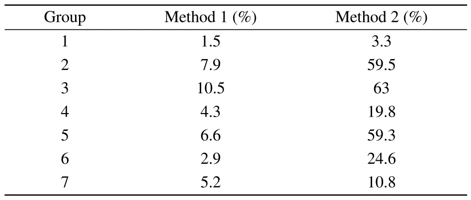
Table 5.Percentage of accuracy improvement of the two methods.
5.Conclusions and perspectives
In this study, the laser interferometric fringe signals are obtained by the NIM-3C gravimeter.The whole falling process is divided into five frequency bands by the Hilbert transformation.The MARMA model is trained according to the number of optimal zero-crossing groups obtained by the honey badger algorithm.The model is used to predict the number of optimal zero-crossing points in each band.The Fourier series fitting method is used to find out the zero-crossing points,and thus, the corresponding time–displacement data are calculated.The independent gravitational acceleration of each frequency band is calculated by the least-squares method,and finally the average value of the gravitational accelerationgof each band is obtained.The Fourier series fitting method reduces the standard deviation of fitted residuals by 53% compared with the windowed second-difference method.Compared to the conventional and improved two-sample zerocrossing detection methods, the accuracy of the gravitational acceleration calculation is improved by 20.6%and 14.1%,respectively.The instantaneous frequency of the laser interference fringe signal increases linearly with time.The number of zero-crossing points then changes accordingly.The number of optimal zero-crossing groups is calculated according to the MARMA prediction model.The gravitational acceleration of the absolute gravimeter is calculated by the number of optimal zero-crossing groups.The accuracy of the gravitational acceleration calculated by test verification is improved by more than 25% compared with that of the fixed number of zerocrossing group method.Therefore, the least-squares fitting with the fixed number of zero-crossing groups has some influence on the accuracy of the gravitational acceleration.The number of optimal zero-crossing groups for each frequency band can be determined by the instantaneous frequency of the laser interference fringe,and selecting the appropriate number of zero-crossing groups can effectively improve the measurement accuracy.
It is shown that the proposed method can effectively improve the accuracy of the gravitational acceleration measurement.It provides a new idea to further improve the accuracy because the optimal algorithm that is used runs slowly and the data of the training set for constructing the prediction model are relatively less.In the future, we will use a large amount of training data to build a more accurate prediction model and improve the calculation speed while ensuring the accuracy.
Acknowledgement
Project supported by the National Key R&D Program of China(Grant No.2022YFF0607504).

- Chinese Physics B的其它文章
- Deterministic remote preparation of multi-qubit equatorial states through dissipative channels
- Direct measurement of nonlocal quantum states without approximation
- Fast and perfect state transfer in superconducting circuit with tunable coupler
- A discrete Boltzmann model with symmetric velocity discretization for compressible flow
- Dynamic modelling and chaos control for a thin plate oscillator using Bubnov–Galerkin integral method
- Analysis of anomalous transport with temporal fractional transport equations in a bounded domain