Investigation of fluid flow-induced particle migration in granular filters using a DEM-CFD method*

HUANG Qing-fu (黄青富), ZHAN Mei-li (詹美礼), SHENG Jin-chang (盛金昌), LUO Yu-long (罗玉龙), SU Bao-yu (速宝玉)

College of Water Conservancy and Hydropower Engineering, Hohai University, Nanjing 210098, China,

E-mail: hqf23@163.com

Investigation of fluid flow-induced particle migration in granular filters using a DEM-CFD method*

HUANG Qing-fu (黄青富), ZHAN Mei-li (詹美礼), SHENG Jin-chang (盛金昌), LUO Yu-long (罗玉龙), SU Bao-yu (速宝玉)

College of Water Conservancy and Hydropower Engineering, Hohai University, Nanjing 210098, China,

E-mail: hqf23@163.com

(Received May 9, 2013, Revised July 8, 2013)

In embankments and earth dams, the granular filter used to protect the base soil from being eroded by the fluid flow is a major safety device. In this paper, the migration mechanism of the base soil through this type of filters with a fluid flow in the base soil-filter system is studied by using the coupled distinct element method and computational fluid dynamics (DEM-CFD) model. The time-dependent variations of the system parameters such as the total eroded base soil mass, the distribution of the eroded particles within the filter, the porosity, the pore water pressure, and the flow discharge are obtained and analyzed. The conceptions of the trapped particle and the trapped ratio are proposed in order to evaluate the trapped condition of the base soil particles in the filter. The variation of the trapped ratio with time is also analyzed. The results show that the time evolutions of the parameters mentioned above are directly related to the gradation of the filter, which is defined as the representative particle size ratio of the base soil to the filter using an empirical filter design criterion. The feasibility of the model is validated by comparing the numerical results with some experimental and numerical results.

base soil-filter system, distinct element method, trapped ratio, representative particle size ratio

Introduction

Embankments and dams are important parts in flood control systems. The safety and the stability of hydraulic structures are important concerns for designers. A substantial amount of related studies indicates that the piping is an important factor that can lead to failure of embankments and earth dams[1]. Since Terzaghi first proposed the famous theory that filters could prevent piping in 1922, the use of filters to protect the base soil from being eroded has been widely adopted in hydraulic engineering designs.

During the past decade, the base soil-filter system was widely studied and several analytical and numerical models were proposed to describe the particlemigration within a base soil-filter system. In the pioneering work by Silveira[2], probabilistic methods were used to examine the migration of the base soil particles through filters, and mathematical formulas were proposed for the filter constriction size distribution in the granular medium under dense conditions. Reddi et al.[3]adopted a numerical model of the filter according to the basic theory of the water flow in a cylindrical tube and found that the permeability coefficient is reduced due to the base soil particle clogging in the filter. Indraratna and Vafai[4]considered the critical hydraulic gradient at which fine particles can move under the limit equilibrium state, and established an erosion model for cohesionless soil based on the conservation of mass and momentum. Locke et al.[5]developed an analytical model based on the work of Indraratna[4]by using a complex 3D void network model to describe the variations of the flow rate, the particle size distribution, the porosity, and the permeability with time in the base soil-filter system. Reboul et al.[6,7]proposed a methodology to compute the constriction size distribution of granular filters, which is an important step to understand and model transportprocesses in granular materials. Frishfelds et al.[8]established a numerical model, which combines the minimization of the dissipation energy rate with the Voronoi discretisation of the particle system to simulate the erosion of fine particles in a granular system. Zou et al.[9]introduced a distinct element method into the study of base soil-filter systems, and established a coupled model to study the base soil-filter system with different filters and a series of useful results were obtained.

The base soil-filter system under a hydraulic load is a complex fluid-structure interaction process involving the ability of the granular media to move under the driving force of the fluid flow, the fluid flow under the influence of granular media, and the migration theory of movable particles in the filter voids. Studies of macroscopic and mesoscopic scales have provided insight about the mechanism of the base soil-filter system, however, not quite enough. The macro model could not describe the migration of base soil fine particles and the clogging of the filter intuitively. The meso model can only describe the distribution of the eroded particles in the filters, without due consideration of the trapped condition of eroded particles in the filters or the change of hydraulic characteristics during the migration of base soil fine particles and clogging of the filter.

In this paper, the coupled distinct element method and computational fluid dynamics (DEM-CFD) model is used to investigate the migration of the base soil in granular filters induced by fluid flow. The time evolutions of the migration and trapped conditions of the base soil in filters with different representative particle size ratios are analyzed. The numerical results are compared with related experimental and numerical results in literature.

1. Coupled DEM-CFD model

The base soil-filter system is considered as a mixture of the particle-phase and the fluid-phase. In the particle-phase, which consists of the base soil particles and the filter particles, the particles are assumed to be spherical. The movement of the particle-phase is modeled by the distinct element method (DEM) based on Newton’s second law of motion and the force-displacement law, while the fluid flow is simulated by the N-S equation that includes the effect of particles. The driving force of the fluid flow is applied to the particles. Thus, the interaction between the particles and the fluid is considered.

1.1Motion of particle-phase

The motion of the particle-phase is solved by the DEM, which was established by Cundall and Strack in 1979. The motion of the particles obeys Newton’s second law as follows:

wherempis the mass of the particle,vpis the velocity of the particle,fgis the gravitational force,fdis the particle-fluid interaction force on the particle,Ipis the moment of inertia,pωis the angular velocity of the particle,fcandMcare the contact force and torque acting on the particle at the contact pointc, respectively.

Fig.1 Contact model

The linear spring-dashpot contact model is adopted in this paper. This model contains the normal and tangential contact components, as shown in Fig.1. The governing equations are as follows:

The equations of the particle motion are integrated using a centered finite difference procedure. The velocity and the position of each particle at every moment can be obtained.

1.2Motion of fluid-phase

The fluid is assumed to be incompressible. TheDarcy’s law is only applicable for the cases of low Reynolds numbers, i.e., with the Reynolds number less than one[10]. It is known that the transient and non-laminar flow plays a more important role in the piping. The Navier-Stokes continuity and momentum equations that take the presence of the particle-phase into account are used in this paper, and are given by:

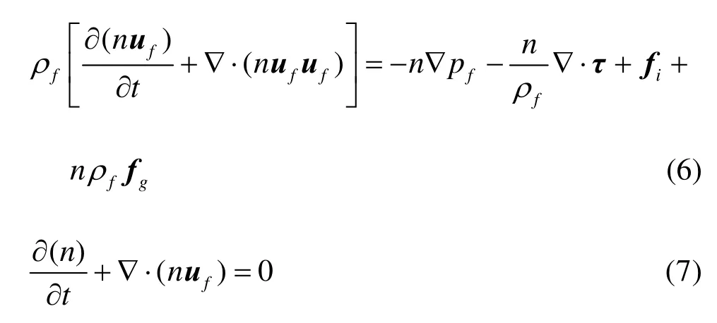
wherefρis the density of fluid,nis the porosity of the particle-phase, ∇ is the gradient operator,ufis the fluid velocity,pfis the fluid pressure,fiis the fluid-particle interaction force on the fluid, andτis the viscous stress tensor defined as follows

in which,fμis the fluid viscosity, ande˙dis the fluid deviatoric strain rate tensor.

The fluid domain is discretized into element cells. The pressure and the velocity of the fluid in each cell are calculated by applying the semi-implicit method for pressure linked equations (SIMPLE).

1.3Fluid-particle interaction and coupled response

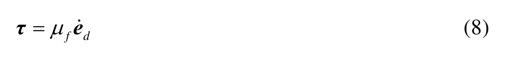
Zhu et al.[11]gave a review of the models for calculating the fluid-particle interaction force. The fluidparticle interaction force on the fluid is given based on the Ergun’s and Wen and Yu’s equations as follow:

whereis the equivalent particle diameter,CDis the drag coefficient, which is a function of the Reynolds number:

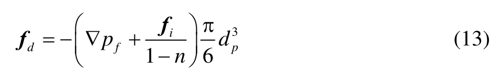
The driving force on the particle by the fluid includes the fluid-particle interaction force and the buoyancy force

The coupled fluid-particle response is calculated as shown in Fig.2, wheretmis the time of calculation,dtis the time step of calculation andtm_set is the time set end of calculation.

Fig.2 Flowchart of coupled fluid-particle calculation

2. Numerical simulation

2.1Particle-phase model

The base soil-filter system is modeled by a cubic sample (0.06 m×0.06 m×0.12 m) within five fixed walls. The model is divided into two parts: the lower part is the base soil, and the upper part is the filter layer. Both parts have a thickness of 0.06 m. The gap-

graded soil is used as the base soil in the model because it is widely used as a core in earth-rock fill dams and it has a high piping tendency under the hydraulic load. The conventional filter design criterion is empirically expressed in terms of the representative ratio of the sizes of the filter particles and the base soil particles

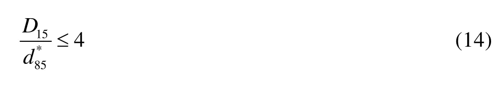
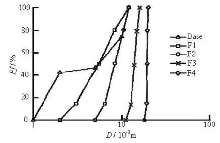
Fig.3 Particle size distribution of the base soil and filters[9]

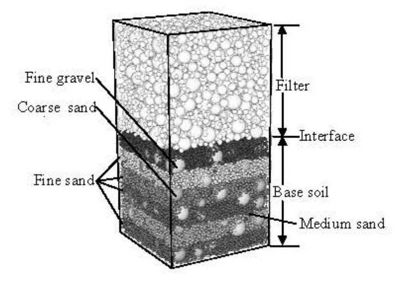
Fig.4 Particle model of base soil-filter system (B-F1)

Following this approach, the mechanism of the base soil-filter system under different filters is analyzed as a function of this ratio. Four filters (F1, F2, F3 and F4) with different representative size ratios are constructed to investigate the mechanism of the base soil-filter system. The representative size ratio of the four filters is gradually increased from F1 to F4. The particle size distributions of the base soil and the four filters are in agreement with those in Ref.[9] , and are shown in Fig.3. Figure 4 shows the particle model of the base soil-filter system, in which the filter is F1. The base soil is divided into four groups based on the particle diameter: the fine gravel (0.010 m-0.012 m), the coarse sand (0.005 m-0.010 m), the medium sand (0.002 m-0.005 m), and the fine sand (0.001 m-0.002 m). The fine sand of the base soil is assigned to six layers with different colors in the model according to thez-position of particles, in order to visually see the migration of the base soil particles. The parameters of the particles and the wall are shown in Table 1.

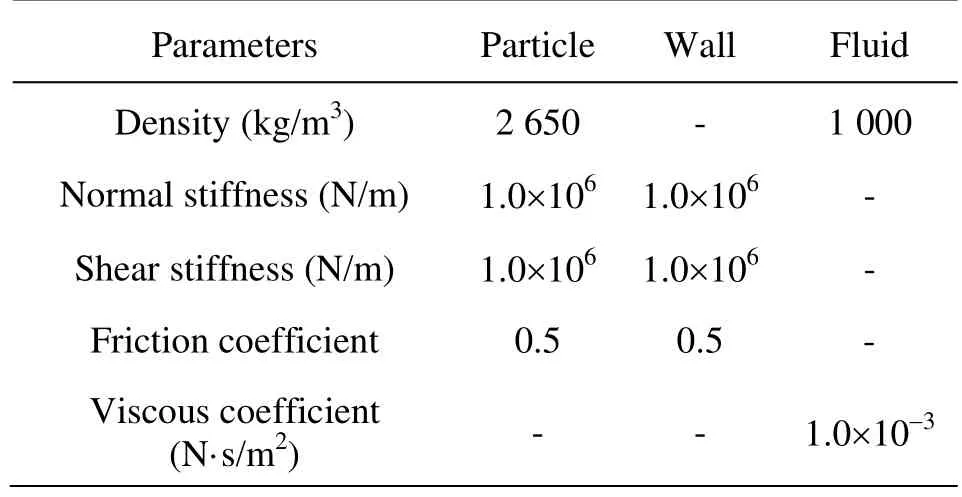
Table 1 Parameters of particle, wall and fluid

2.2Fluid-phase model

The simulation domain is divided into a 4×4×8 fluid grid along thex-,y- andz- directions. The hydraulic pressure is added to the bottom of the model, while the top of the model is set as the outflow boundary with zero pressure. The other walls are set as slip walls. The fluid parameters are shown in Table 1.

2.3Simulation case

The main purpose of the filter is to prevent the base soil from being eroded. The filter is designed according to the criterion expressed in terms of the representative size ratio used in the construction practice. In order to investigate the erosion process of the base soil under different filters, four groups of analysis cases are designed with different representative size ratios, labeled as “B-F1”, “B-F2”, “B-F3” and “B-F4”, as shown in Table 2. The calculation time is set to 0.3 s in order to investigate the influence of time on the erosion of the base soil. In Ref.[9], a time of 0.04 s was used.

3. Simulation results and discussions

The migration and trapped conditions of base soil particles in different filters with different representative size ratios are studied. The results are discussed in the following sections: including the particle distributions of the base soil-filter system at the end of simulation, the mass of the total eroded base soil, the distribution of the eroded particles within the filter, the trapped ratio, the porosity, the pore water pressure, and the flow discharge.

3.1Particle distributions at the end of simulation

Figure 5 shows the particle distributions of the base soil-filter system at the end of the simulation.The bold lines mark the divisions between the six layers of the fine base soil at the initial time. Figure 6 shows the velocity vectors of the base soil particles at the end of the simulation.

Table 2 Analysis cases for numerical models

Fig.5 Positions of particles att=0.3s

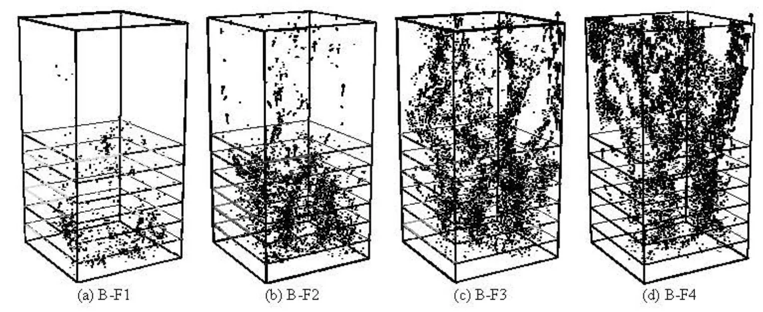
Fig.6 Velocities of base soil particles att=0.3s

Comparing Fig.5 with Fig.4, it can be seen that the positions of the base soil particles under different filters at the end of the simulation are quite different. In the cases of B-F1 and B-F2, whose filters are effective according to the filter design criterion, the eroded base soil particles are much fewer than those in cases B-F3 and B-F4. From Fig.6, one can see that the number of moveable particles increases with the increase of the representative size ratio. Although some base soil particles transport in the filter and may be transported completely through the filter in cases B-F1 and B-F2, but most of the eroded particles in the filter near the interface are unmovable which means that the interface becomes stable. Most of the eroded base soil particles in the filter are movable in cases B-F3 and B-F4, and are mainly concentrated in some connectivity voids of the filter. Some channels from which the base soil can erode out of the filter are formed, which means that the filter cannot protect the base soil from being eroded. From the above observations, it can be concluded that: (1) the probabilities of the base soil penetrating into the four filters are not the same; the greater the representative size ratio is, the more base soil particles will be eroded, (2) when the representative size ratio satisfies the criterion, the filter could cause the base soil to clog the interface, which means that the filter can prevent the base soil from being eroded, (3) when the representative size ratio does not sa-tisfy the criterion, the base soil particles will migrate in the pore network of the filter, and not many of them clog the filter, which means that the filter cannot prevent the base soil from being eroded.

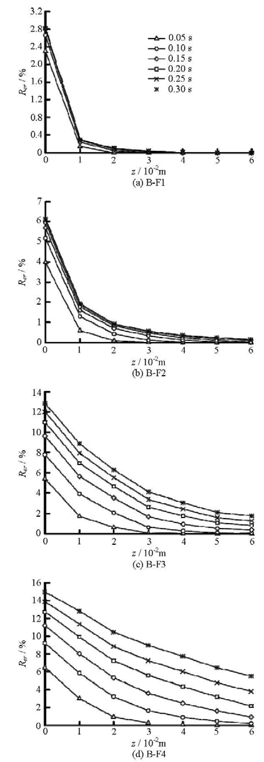
Fig.7 The evolutions of the distribution of the eroded ratio in the filter

3.2The time evolution of the distribution of the eroded

ratio

In order to study the distribution of eroded particles at different depths of the filter, the eroded ratio

Rer(z) is defined as the percentage of the mass of the eroded particles which are eroded over the distancezfrom the interface, over the total mass of the base soil

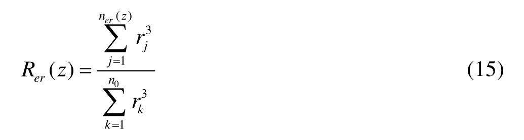
wherener(z) is the number of particles eroded over the distancezfrom the interface in the filter,rjis the radius of the eroded particle,n0is the number of the base soil particles,rkis the radius of the base soil particle.Rer(0), represents the ratio of the total eroded particles into the filter, and is called the total eroded ratio.Rer(6), represents the ratio of the eroded particles that move out of the filter, and is referred to as the loss ratio. Figure 7 shows the variations of the distribution of the eroded ratio with time under different filters. It can be seen that: (1) In cases B-F1 and B-F2, the evolutions of the distribution are similar. The eroded ratios diminish with the distance from the interface at any simulation time. The distribution at any time follows a negative exponential distribution, as is identical to the experiment results in Ref.[12] that is referenced in Ref.[13]. The eroded ratio at any depth of the filter tends to increase gradually with time and finally reach a stable value, which indicates that the base soil can be prevented from being eroded under the protection of filters. (2) In cases B-F3 and B-F4, the evolutions of the distribution are different from those in cases B-F1 and B-F2. Most of the time, the distribution follows a negative exponential distribution, but tends to be linear at the end of the simulation in the case of B-F4. The eroded ratio at any depth of the filter increases gradually with time and has no trend to become stable, which indicates that the base soil will be eroded continually with time.

3.3The time evolution of the total eroded ratioFigure 8 shows the variations of the total eroded ratioRer(0) with time under different filters. It can be seen that:

(1) In the cases of B-F1 and B-F2, the evolution processes can be divided into three stages:

(a) In the initial stage, the total eroded ratio increases quickly, which means that the base soil parti-cles are eroded into the filter quickly. This is due to the larger size and porosity of the filter as compared to those of the base soil at the base soil-filter interface, thereby, the base soil can be eroded into the filter quickly under the driving force of the fluid flow.

(b) During the developing stage, although the total eroded ratio increases, the increasing rate is reduced slowly and tends to be zero. This is because the particles are trapped by the filter and clog the filter voids, which will minimize the size of filter voids and make it more difficult for subsequent particles to pass through the voids.

(c) At the stable stage, the total eroded ratio becomes stable, and does not change with time. The total eroded ratios reach 2.8% and 6.1% in cases B-F1 and B-F2, respectively. This shows that the base soil can be prevented from a progressive erosion under the protection of filters F1 and F2.

(2) In the cases of B-F3 and B-F4, the evolution processes only contain the first two stages compared to those of B-F1 and B-F2. The initial stage is similar to that in cases B-F1 and B-F2. In the developing stage, the total eroded ratio increases and the increasing rate is reduced slowly and tends to be constant but not zero, which means that the process of the base soil being eroded into the filter will continue and cannot be stopped.

Fig.8 The evolution of total eroded ratio

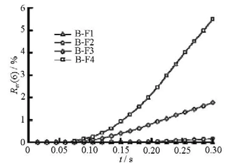
Fig.9 The evolution of loss ratio

3.4The time evolution of loss ratio

Figure 9 shows the evolution of the loss ratioRer(6). The loss ratios in cases B-F1 and B-F2 are very small and from the evolution of the total eroded ratio illustrated in Section 3.3, it can be deduced that the loss ratio will reach a stable value with time. This means that after a period of time, there will be no more particles lost from the filter. The loss ratios in cases B-F3 and B-F4 gradually increase with time, and the increasing rate of the loss ratio will be con- stant after a period of time. Also, from the evolution of the total eroded ratio, it can be deduced that the loss ratio will continually increase with time. The time evolution of the loss ratio in cases B-F3 and B-F4 ag- rees with the experiment results of ineffective filters in Ref.[14]. 3.5The time evolution of trapped ratio

From the above analysis, it can be seen that with the increase of the representative size ratio, the filter’s ability to protect the base soil from being eroded decreases. In order to represent the capacity of protection by the filters with different representative size ratios more directly, the “trapped particle” is defined within this model. If the increment of thez-coordinate of the particle’s position is less than 5.0×10–6m in 0.003 s, then the particle will be considered as a “trapped particle”. Even when a particle is static, because of the characteristics of the distinct element method, it is uncommon for the velocity of a particle to be absolutely zero, its velocity will fluctuate within a small range. The corresponding critical velocity of a “trapped particle” is only about 0.1% of the interstitial velocity. It can be considered that the critical velocity is reasonable for the identification of the “trapped particle”.

According to the definition of the trapped particle, the “trapped ratio” of the eroded particles in a filter can be defined as

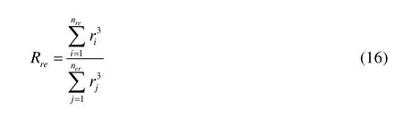
wherenreis the number of the trapped particles in the filter,neris the total number of the eroded particles, andiris the radius of the trapped particle.

Figure 10 shows the variation of the trapped ratio with time. The trapped ratio increases gradually with time. Once one particle is trapped in the filter void, the trapped particle will become a new part of the fi- lter, and the local filter void will be smaller, for the subsequent trapping of particles.

(1) In the cases of B-F1 and B-F2, the trapped ratio increases quickly with time. The trapped ratio reaches 99% att=0.20 s in the case of B-F1, while the trapped ratio reaches 93% att=0.30 s in the caseof B-F2. Both the trapped ratios are higher than 90%.

(2) In the cases of B-F3 and B-F4, although the trapped ratio increases with time at the beginning, the increasing rate is smaller compared to that in cases B-F1 and B-F2. The trapped ratio is always relatively low over time, reaching only 39% and 14 % in cases B-F3 and B-F4, respectively. This shows that the filters F3 and F4 cannot effectively protect the base soil from being eroded.

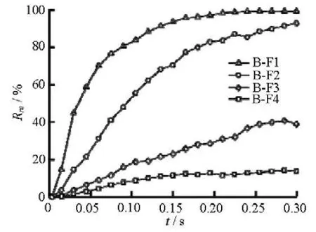
Fig.10 The evolution of trapped ratio

The conclusion drawn from the analysis of the trapped ratio is consistent with that drawn in former sections. The trapped ratio can reflect the capability of protection by the filter very well. The lower the capability, the lower the trapped ratio will be.

3.6The time evolution of porosity

The evolution of the porosity is closely related to the migration of the base soil particles in filters. It can reflect the relationship between the amounts of particles penetrated into the soil layer, and that of particles which have moved out of the soil layer.

Figure 11 shows the evolution of the porosity with time in the base soil and filter. Only the cases of B-F1 and B-F3 are given due to space limitations (BF2 is similar to B-F1, and B-F4 is similar to B-F3). The positions of the eight layers are illustrated in Fig.11(c). Due to the effect of the wall boundary, the number of particles per unit volume near the wall is smaller than that inside the body, so the initial porosities of BL1 and BL4 are little larger than those of BL2 and BL3.

(1) In the case of B-F1, the porosity changing process over time can be divided into three stages, which correspond to the evolution of the total eroded ratio with time as mentioned above: (1) the initial stage, in which the porosity of BL4 (the base soil side of the interface) increases quickly with time, and the porosity of FL1 (the filter side of the interface) decreases quickly, (2) the developing stage, in which the porosity of BL4 increases slowly with time and after a period of time, it begins to decrease with time. The porosity of FL1 continues to decrease and the decreasing rate gradually reduces with time. This is because the former trapped particles reduce the void of the filter, and makes it more difficult for the subsequent particles to pass through the void, but the particles in BL3 continually penetrate into BL4 under the driving force of the fluid flow. After a period of time, the amount of particles penetrated into BL4 will be greater than those eroded into FL1, (3) the stable stage, the porosities of BL4 and FL1 are no longer changing over time. In the three stages, the porosities of FL2, FL3, and FL4 are nearly invariable with time, which means that there are only a small amount of the base soil eroded into FL2, FL3 and FL4. The porosities of BL2 and BL3 only change a little with time, while the porosity of BL1 gradually increases with time and reaches a stable value at the end of the simulation. This is because when the particles move out of BL3, the particles in BL2 will penetrate into BL3 under the fluid flow, which reaches a balance. However, for BL1, no particles move in. The phenomena can be seen in Fig.5.

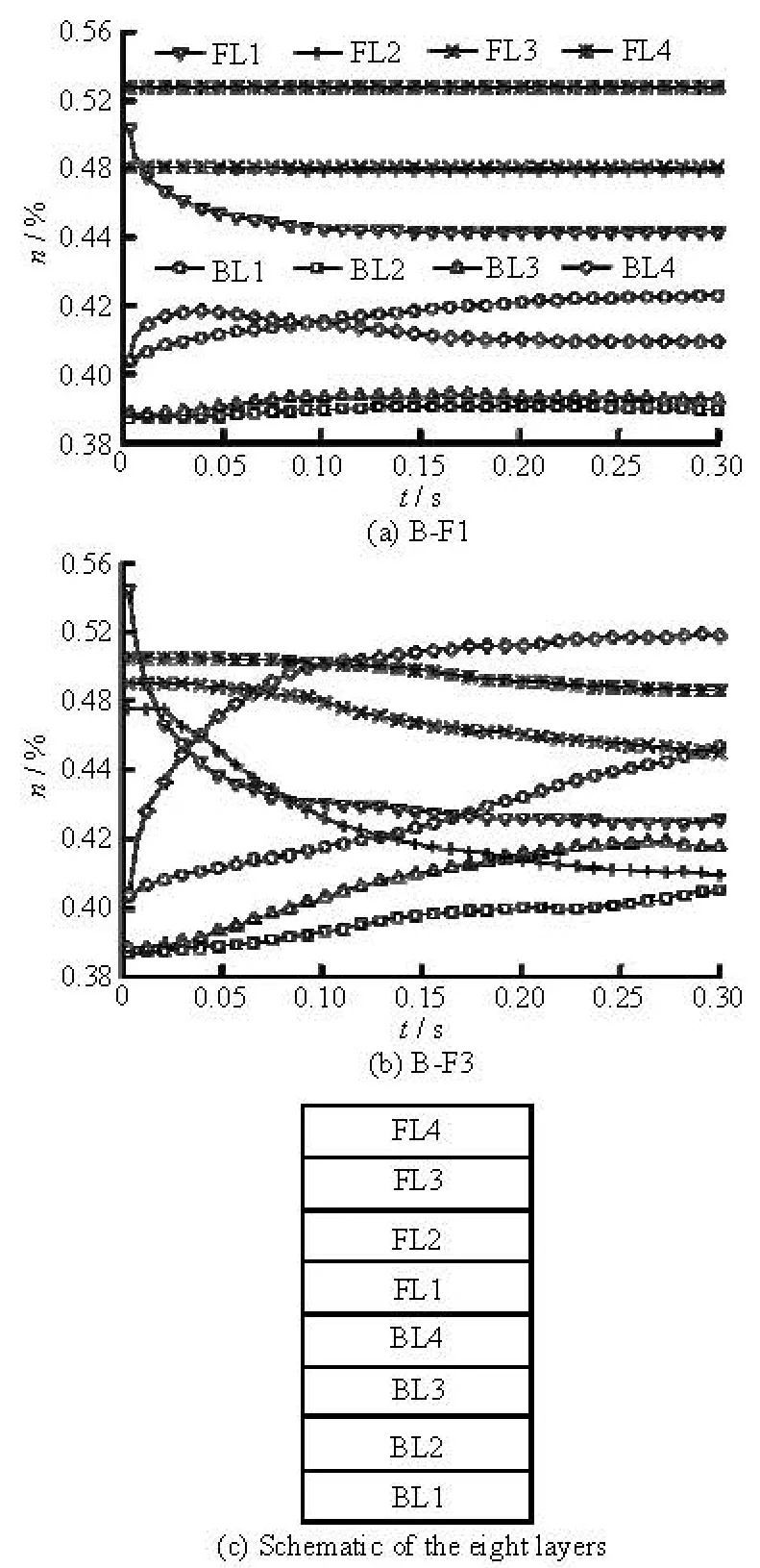
Fig.11 The evolution of porosity

(2) In the case of B-F3, the porosities of FL1,FL2, FL3, and FL4 decrease over time, while the porosities of BL1, BL2, BL3, and BL4 gradually increase over time, which means that the base soil is eroded gradually with time, and there is no trend to stop.

3.7The time evolution of pore water pressure

The variations of the pore water pressure with the flow path reflect the water head loss in the system, which is directly related to the permeability of the soil. The greater the pressure gradient, the smaller the permeability of the soil will be.

Fig.12 The evolution of pore water pressure (PWP)

Figure 12 shows the evolution of the water pressure with time in the base soil and the filter. Here, only the cases of B-F1 and B-F3 are given due to space limitations (B-F2 is similar to B-F1, and B-F4 is similar to B-F3). Att=0.003 s, the pressure gradient in the base soil is greater than that in the filter layer in both cases, which means that most of the head loss is borne by the base soil at the beginning.

(1) In the case of B-F1, the pressure in the base soil gradually increases with time, while the pressure in the filter is nearly invariable with time, except in locations near the interface. That is because the porosity of BL1 is increased with time, and the permeability of BL1 is increased correspondingly according to the Kozeny-Carman equation which leads to the increase of the pressure atz=0.0075 m. The pressure gradient is almost invariable from 0.0075 to 0.0525 m corresponding to the invariability of the porosities of BL2 and BL3. The pressure gradient at the interface is increased, corresponding to the decrease of the porosity for FL1.

(2) In the case of B-F3, the pressure in both the base soil and the filter is increased with time. At the end of the simulation, the pressure gradient in the base soil and the filter are almost the same. This corresponds to the evolution of the porosity as is analyzed in Section 3.6. With a large amount of the base soil eroded into the filter, the permeability of the base soil is increased, while the permeability of the filter is decreased.

The eroded base soil going into the filter will result in an increase of the pressure in the filter, which means the proportion of the head loss borne by the filter becomes larger, as is consistent with the experiment results in Ref.[15].

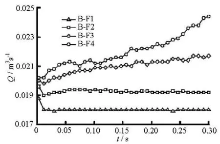
Fig.13 The evolution of flow discharge

3.8The time evolution of discharge

Figure 13 shows the evolution of the discharge (Q) with time. In cases B-F1 and B-F2, the discharge is decreased at the beginning, and then tends to be stable. In the model by Reddi[3], the discharge in an effective filter is shown to increase initially, and then decrease with time, and the initial increase is due to some base soil particles being washed out through the filter. In our model, only a few particles will be washed out through the filter at the end of simulation, so there is no initial increase in our model. In cases B-F3 and B-F4, the discharge is initially decreased due to the penetration of the base soil into the filter. Following the initial decrease, the discharge gradually increases with time while the base soil particles are washed out of the filter. The increase stage is consistent with the prediction by Reddi[3]in an ineffective filter. The flow discharge fluctuates during the process in cases B-F3 and B-F4, which is due to the continuous migration of the eroded particles in the filter. The porosity of the fluid cell varies during the process, sometimes a decrease of the porosity of some fluid cells may lead to the decrease of the flow discharge. While the total porosity is increased during the process in cases B-F3 and B-F4, the flow discharge is increased in general.

4. Conclusions

The coupled DEM-CFD model is used to investigate the migration mechanism of the base soil through filters under a hydraulic load. Four filters with different representative size ratios are designed in order to analyze the influence of the representative size ratio on the migration and trapped condition of the base soil. The simulation results can be summarized as follows:

(1) The representative size ratio has a great influence on the effectiveness of the filter. With the increase of the representative size ratio, the trapped ratio is decreased, which means that the filter’s capability of preventing the base soil from being eroded is decreased. The effectiveness of the filter, as identified by our model, agrees with the empirical filter criterion. The filters F1 and F2 are effective, while filters F3 and F4 are ineffective.

(2) When a filter is effective, there will be only a small amount of eroded particles that can move in the filter, and most of the particles will be trapped in the filter not far from the interface. The eroded ratio is reduced along the direction from the interface to the filter in a negative exponential distribution. The discharge will initially decrease and then reach a stable value.

(3) When the filter is ineffective, the eroded particles will migrate continually in the void network of the filter and move out of the filter. The discharge will initially decrease and then increase with time.

Some simulation results are compared to the related experimental or numerical results. The results show that the coupled DEM-CFD model is feasible. The model can visually model the migration and trapped condition of the base soil in filters under a fluid flow in a base soil-filter system, and appears to be a very promising tool for research of the erosion mechanism in a base soil-filter system.

[1] FOSTER M., FELL R. and SPANNAGLE M. The statistics of embankment dam failures and accidents[J].Canadian Geotechnical Journal,2000, 37(5): 1000-1024.

[2] SILVEIRA A. An analysis of the problem of washing through in protective filters[C].Proceeding of 6th International Conference of Soil Mechanics and Foundation Engineering.Toronto, Canada, 1965, 551-555.

[3] REDDI L. N., MING X. and HAJRA M. G. et al. Permeability reduction of soil filters due to physical clogging[J].Journal of Geotechnical and Geoenvironmental Engineering,2000, 126(3): 236-246.

[4] INDRARATNA B., VAFAI F. Analytical model for particle migration within base soil-filter system[J].Journal of Geotechnical and Geoenvironmental Engineering,1997, 123(2): 100-109.

[5] LOCKE M., INDRARATNA B. and ADIKARI G. Time-dependent particle transport through granular filters[J].Journal of Geotechnical and Geoenvironmental Engineering,2001, 127(6): 521-529.

[6] REBOUL N., VINCENS E. and CAMBOU B. A statistical analysis of void size distribution in a simulated narrowly graded packing of spheres[J].Granular Matter,2008, 10(6): 457-468.

[7] REBOUL N., VINCENS E. and CAMBOU B. A computational procedure to assess the distribution of constriction sizes for an assembly of spheres[J].Computers and Geotechnics,2010, 37(1-2): 195-206.

[8] FRISHFELDS V., HELLSTROM J. G. I. and LUNDSTROM T. S. et al. Fluid flow induced internal erosion within porous media: modelling of the no erosion filter test experiment[J].Transport in Porous Media,2011, 89(3): 441-457.

[9] ZOU Y.-H, CHEN Q. and CHEN X.-Q. et al. Discrete numerical modeling of particle transport in granular filters[J].Computers and Geotechnics,2013, 47: 48-56. [10] SHAMY U. E., AYDIN F. Multiscale modeling of flood-induced piping in river levees[J].Journal of Geotechnical and Geoenvironmental Engineering,2008, 134(9): 1385-1398.

[11] ZHU H. P., ZHOU Z. Y. and YANG R. Y. et al. Discrete particle simulation of particulate systems: Theoretical developments[J].Chemical Engineering Science,2007, 62(13): 3378-3396.

[12] SAIL Y., MAROT D. and SIBILLE L. et al. Suffusion tests on cohesionless granular matter: Experimental study[J].European Journal of Environmental and Civil Engineering,2011, 15(5): 799-817.

[13] SARI H., CHAREYRE B. and CATALANO E. et al. Investigation of internal erosion processes using a coupled dem-fluid method[C].PARTICLES 2011 II International Conference on Particle-Based Methods-Fundamentals and Applications.Barcelona, Spain, 2011, 1-11.

[14] ZHANG Gang. Researches on meso-scale mechanism of piping failure by means of model test and PFC numerical simulation[D]. Doctoral Thesis, Shanghai, China: Tongji University, 2007(in Chinese).

[15] ZHOU Jian, BAI Yan-feng and YAO Zhi-xiong. Mesoscale model test on filter prevention of piping-typed soils[J].Journal of Hydraulic Engineering,2010, 41(4): 390-397(in Chinese).

* Project supported by the National Natural Science Foundation of China (Grant Nos. 51079039, 51009053 and 50779012).

Biography: HUANG Qing-fu (1985-), Male, Ph.D. Candidate

ZHAN Mei-li,

E-mail: zhanmeili@sina.com