Motion Planningfor MinimizingBase Disturbance of Space Manipulators

JI Lu（纪 路），ZHOU Dongsheng（周东生），ZHANG Qiang（张 强）

Key Laboratory of Advanced Design and Intelligent Computing （Dalian University），Ministry of Education，Dalian 116622，China

Introduction

A spacecraft system which is mounted a robotic manipulators holds inestimable value for business and defense.Since the property of momentum conservation during the operation of space manipulators，the motion of manipulators could disturb the position and attitude of its base and make the end-effector miss the destination［1］.Generally，thrusters，orthogonal reaction wheels or control moment gyroscopes are utilized to counteract the disturbance，but in this paper the base disturbance should be minimized with planning the motion of space manipulators.

There are many related work finished by predecessors.Dubowsky et al.proposed enhanced disturbance map（EDM）［2-3］method，which could illustrate the maximal and the minimal base disturbances with regard to different orientations of motion of space manipulators by maps clearly.Yoshida et al.addressed the zero reaction maneuver（ZRM）concept［4］，which could plan the motion of space manipulators without base disturbance，despite it only acted on certain manipulators with dynamics redundancy.Yamada employed a “calculus of variations”to planning the motion of joints［5］，for arbitrarily changing the attitude of base.Suzuki and Nakamura developed Yamada's method，and then proposed the optimal spiral motion［6］，but this method was constrained by dynamic singularity.Papadopoulos et al.［3］used a method of parameter optimization，but it was only exampled by 2-DOF space manipulators.

In this paper，aplanning method，which is inspired by previous labors，is proposed to plan the motion for minimizing base disturbance of 6-DOF space manipulators.The paper is organized as follows.Section 1 derives the direct and inverse equations of manipulators system.Section 2 introduces the quaternion expression.Section 3 parameterizes the joint motion and system state and transforms the planning problem to optimal problem.Section 4introduces the detail steps of simulated annealing particle swarm optimization （PSO）algorithm.Section 5 shows the computer simulation results.In the final，section 6make a conclusion for the presented work.

1 Modeling and Kinematics

There is no point-to-point relationship between joint space and cartesian space in space manipulators system，because the position and orientation of end-effector depend not only on the geometrical configuration of manipulators，but also on the history of motion of manipulators.To depict this relationship Umetani and Yoshida proposed the conception of generalized Jacobian matrix（GJM）［7］，which expressed the system function by velocity-level kinematical equation instead of position-level ones.The model of space manipulators is shown in Fig.1.

Fig.1 The model of 6-DOF space manipulators

In the following of the paper，many symbols in the formulas are shown in Table 1.

Table 1 Symbol and notation

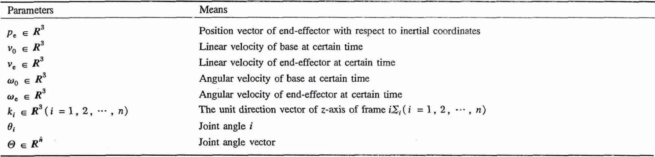
Table 1 continued

1.1 Equation of kinematics—GJM

Position equation of end-effector is shown in Eq.（1），

then differentiate Eq.（1）with respect to time，

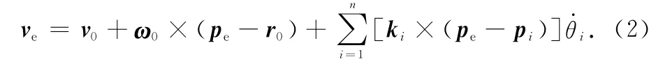
And the angular velocity of end-effector is

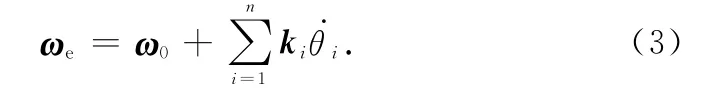
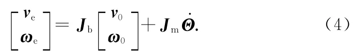
The kinematical equation of free-flowing manipulators system is as follows：

Since the Law of Momentum Conservation，this leads to

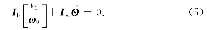
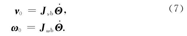
According to Eq.（5），v0andω0can be solved as

This equation can be divided into linear velocity part and angular velocity part，which is as follows

At last，substituting Eq.（6）into Eq.（4），the equation is yielded

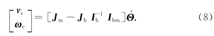
J＊（Ψb，Θ，mi，Ii）is the so called GJM，which represents the feature of kinematics of the whole space manipulators system.It is determined by not only the geometrical parameters of each link but also the inertia properties of the total system.

1.2 Inverse kinematics—Theory of Screws

For meeting the multi-solutions property of manipulators inverse kinematics，this paper combines Theory of Screws［8］and Paden-Kahan sub-problem［9］to solve the inverse kinematics problem［10］.

We use exponential coordinate instead of rectangular coordinate system because this method can regard rotation as a vector.If the initial position of a particle relative to a fixed axis is g（0）in this coordinate system，the terminal position is g（θ）after the particle rotation about this axis：

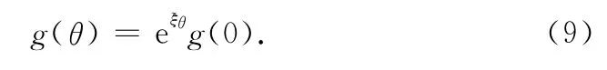
The physical meaning of exponential coordinate system is pretty clear.In this paper，the end-effectorrotates continuously about several sequential joints through anglesΘ＝［θ1，θ2，…，θn］radians，and then the terminal position can be obtained：

1.3 Solution of inverse kinematics

We assume the manipulators hold at least three continuous joint axes intersecting to one point pcross（this is a common property of industrial manipulators）.In this case，the position of point pcrosswith regard to rectangular coordinate system is unchanged during it rotation about arbitrary axis among this three（e.g.，joints 4，5，and 6 intersect to point pcross）：

and then Eq.（10）can be expressed as follows：

Both sides of equation above can be expanded into a threevariable linear equation system，which can be utilized to calculate the angles of joints 4，5，and 6.In the same way，this paper can get the values of the rest joints as well.

Since our goal of planning is to make the final state of base nearly equal its initial state，this paper can regard the final state of base as the fixed-base manipulators and calculate its inverse kinematics as above.

2 Quaternion Expression of Attitude

Chou used unit quaternion，which was a proper parametric representation without singularities，to describe finite rotations［11］.The relationship between the time differentiation of quaternion and the angular velocity can be established as follows：

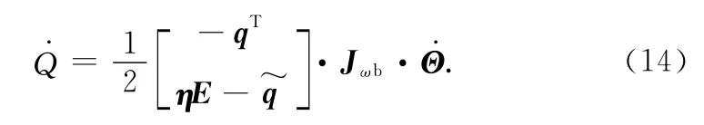
Substituting Eq.（7）into Eq.（13），the variation rate of attitude can be derived：

For two coordinate frames，their orientations are described by Q1，and Q2respectively，and the orientation errors are given byδηandδq［12］：

3 Description of Motion Planning Problem Based on Direct Kinematics

3.1 Parameterization of joint motion

For obtaining smooth curve，this paper utilizes the polynomial function to describe the joint motion.

where t0and tfare the initial time and the terminal time，respectively.

Substituting Eq.（17）into the equations ofθi（t），（t），and（t），one can obtain ai1，ai2，ai3，ai4，ai5by（θi0，θid，ai6，ai7，Δi1，Δi2），whereθi0andθidare the initial and the desired angles of joint i，respectively.At last，only two parameters（ai6，ai7）are remained in every joint motion function.

3.2 Equation of system state

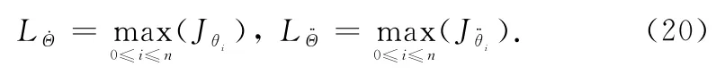
In this paper，the attitude and position of spacecraft

can be calculated by numerical integration：

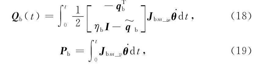
where，J is the Jacobian formula and m represents the intertia of the spacecraft.The goal of motion planning is to make the distance of the final and the initial／desired state close to zero.

3.3 Limitation of joint motion

For more practical use of this motion planning method，the boundary of joint velocities and accelerations must be constrained：

4 Solution of Motion Planning Problem by Optimization Algorithm

4.1 Definition of objective function

Considering the dynamics coupling relationship between manipulators and base，the motion of manipulators could disturb the position and attitude of free-flowing base which supports the manipulators.So the objective function is defined as：

whereδqb，δpb，LΘ·，and LΘ··are defined above；Kq，Kp，KΘ·，and KΘ··are determined by the accuracy requirement；andThe flowchart of objective function calculation is shown in Fig.2.

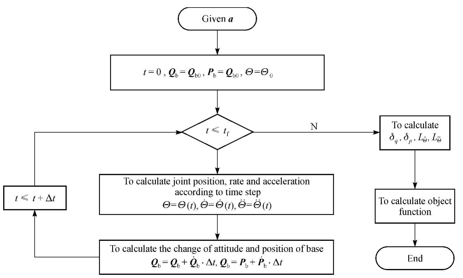
Fig.2 The flowchart of objective function calculation

4.2 Solution of the motion planning

According to the property of PSO algorithm，the position of each particle with regard to higher dimensional space could refer to a group of Lagrange multiplier a.Because the objective function is determined by a，this paper can use a position of a particle，which could calculate the minimal objective function value，to express the solution of motion planning problem.The steps are as follows.

Step 1 Set the initial temperature：

Step 2 The first function of the pair of functions is determined by piand t0：

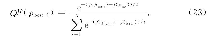
Step 3 Adopting the Roulette Algorithm，the larger value of QF（pbest＿i）is，the more opportunities that the corresponding pbest＿ican be elected to be gbest.As long as the convergence of the algorithm，pbest＿ithat corresponds to the larger QF（pbest＿i）has larger opportunity to be elected and vice versa.

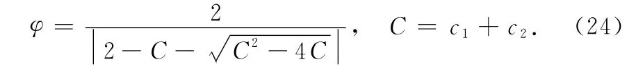
Step 4 Add the compressibility factor and remove the inertia weight，The position equation is unchanged and the velocity equation is as follows：

Step 5 Among the PSO，the second function of the pair of functions will be inserted that generally be called Annealing Function：

whereλis an annealing constant.

5 Simulation Results

The parameters of the whole system are shown in Tables 2and 3.The simulation environment is Matlab 2010a with a toolbox“Spacedyn”that programed by Shimizu et al.［13］

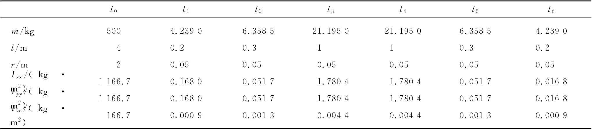
Table 2 Mass properties of each body

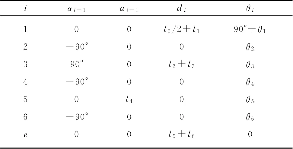
Table 3 The D-H parameters of the whole system

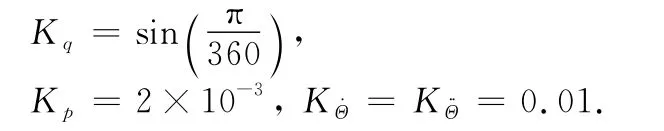
The coefficients of accuracy are as follows：

The initial state of system and the position of end-effector are：

The parameters of the simulated annealing PSO algorithm are shown in Table 4.

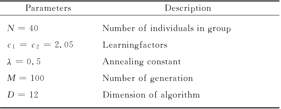
Table 4 The parameters of the simulated annealing PSO algorithm

Figure 3shows the relationship between the value of objective function and the number of generation.The corresponding curves of attitude and position of base spacecraft are shown in Figs.4and 5，respectively.

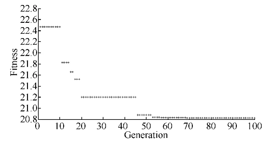
Fig.3 Variation of the fitness

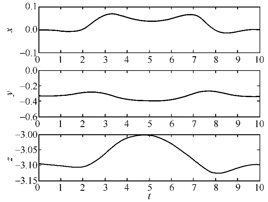
Fig.4 Curves of base position

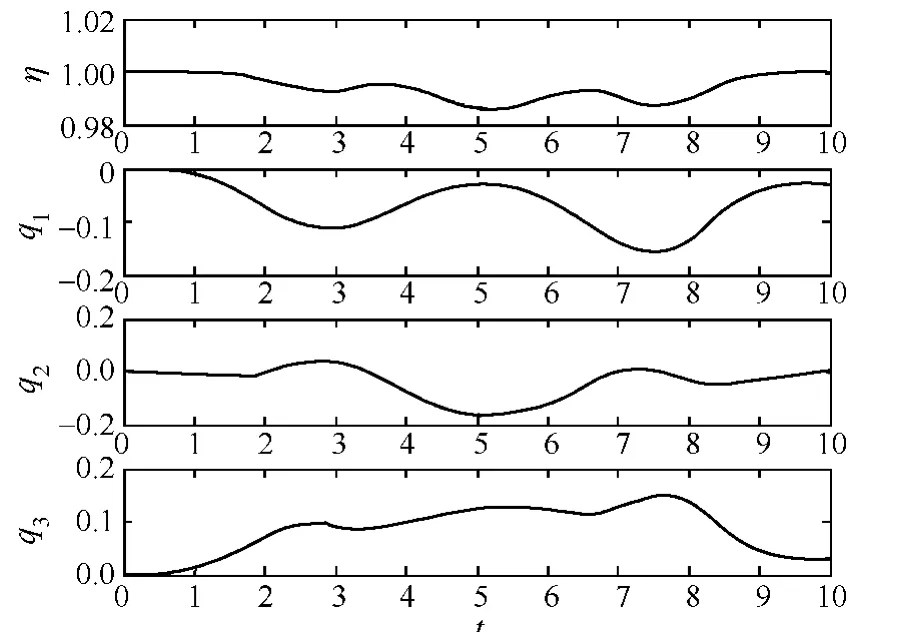
Fig.5 Curves of base attitude

The optimal aand the value of fitness are：

We can notice that the fitness is an invariable value after generation 70.The final position and attitude of spacecraft are［PbfQbf］＝［-0.015 -0.305 9 -3.086 3 0.999 4 0.013 3 -0.010 6 0.033 0］.

In the formula，b represents the “base”of the manipulator；f represents the“final”position of the moving manipulator.The first three numerical valuse are the positions which represent coordinates of x， y， z，respectively.And，the remaining four numerical values are quaternion of the terminal posture of the manipulator.

6 Conclusions

In this paper，a 6-DOF space manipulators is modeled and the plan of motion of minimizing base disturbance is provided.The objective function has quite a few extreme points due to the complexity of motion equation of 6-DOF space manipulators.Particularly，there are several suboptimal solutions close to the globally optimal solution.General algorithm hardly searches the best result.For better dealing with this problem，this paper takes advantage of a simulated annealing PSO algorithm.From the simulation results，one can see that this algorithm can rapidly converge to a better solution.

［1］Huang P F，Xu Y S，Liang B.Dynamic Balance Controlof Multi-arm Free-Tloating Space Robots［J］.International Journal of Advanced Robotic Systems，2005，2（2）：117-125.

［2］Dubowsky S，Torres M.Path Planning for Space Manipulators to Minimize Spacecraft Attitude Disturbances ［C ］.Proceedings of the IEEE International Conference on Robotics and Automation，Sacramento，CA，1991：2522-2528.

［3］Papadopoulos E，Dubowsky S.Coordinated Manipulator／Spacecraft Motion Control for Space Robotic Systems［C］.Proceedings of the IEEE International Conference on Robotics and Automation，Sacramento，CA，1991：1696-1701.

［4 ］Yoshida K， Hashizume K， Abiko S.Zero Reaction Maneuver：Flight Validation with ETS-VII Space Robot and Extension to Kinematically Redundant Arm［C］.Proceedings of the IEEE International Conference on Robotics and Automation，Piscataway，USA，2001：441-446.

［5］Yamada K.Arm Path Planning for a Space Robot［C］.Proceedings of the IEEE／RSJ International Conference on Intelligent Robots and Systems，Yokohama，Japan，1993：2049-2055.

［6 ］Suzuki T， Nakamura Y.Planning Spiral Motion of Nonholonomic Space Robots［C］.Proceedings of the IEEE International Conferences on Robotics and Automation，Minneapolis，Minnesota，1996：718-725.

［7］Umetani Y，Yoshida K.Resolved Motion Rate Control of Space Manipulators with Generalized Jacobian Matrix［J］.IEEE Transactions on Robotics and Automation，1989，5（3）：303-314.

［8］Murray R M，Li Z，Sastry S S.A Mathematical Introduction to Robotic Manipulation［M］.Florida：CRC Press，1994：110-140.

［9 ］Campion G，Bastin G， D'Andréa-Novel B.Structural Properties and Classification of Kinematic and Dynamic Models of Wheeled Mobile Robots［J］.IEEE Transactions on Robotics and Automation，1996，12（1）：47-62.

［10］Tan Y S，Xiao A P.Extension of the Second Paden-Kahan Sub-problem and Its'Application in the Inverse Kinematics of a Manipulator ［C］.IEEE Conference on Robotics，Automation and Mechatronics，Chengdu，China，2008：379-381.

［11］Chou J C K.Quaternion Kinematic and Dynamic Differential Equations ［J］.IEEE Transactions on Robotics and Automation，1992，8（1）：53-64.

［12］Yuan J S C.Closed-Loop Manipulator Control Using Quaternion Feedback［J］.IEEE Journal of Robotics and Automation，1988，4（4）：434-440.

［13］The Spacedyn：a MATLAB Toolbox for Space and Mobile Robots［EB／OL］.（2006-07-20）［2014-09-28］.http：／／www.astro.mech.tohoku.ac.jp／spacedyn／.