Numerical Modeling and Prediction of the Effectof Cooling Drag on the Total Vehicle Drag

A. Rustem Aslan, Kerem Anbarci, M. Berkay Acikgoz, Omur Icke, Ozgur Aslan, Cenk Dinc

(1. Istanbul Technical University, Maslak, Istanbul 34469, Turkey; 2. AES-Aero Engineering Ltd., Turkey; 3. FORD Motor Company, Turkey)



Numerical Modeling and Prediction of the Effectof Cooling Drag on the Total Vehicle Drag

A. Rustem Aslan1,*, Kerem Anbarci2, M. Berkay Acikgoz2, Omur Icke3, Ozgur Aslan3, Cenk Dinc3

(1. Istanbul Technical University, Maslak, Istanbul 34469, Turkey; 2. AES-Aero Engineering Ltd., Turkey; 3. FORD Motor Company, Turkey)

The effect of the engine cooling on the total drag is evaluated by numerical analyses using CFD methods for a light commercial vehicle. The numerical mesh includes both exterior and interior (engine compartment, under hood components) parts of the vehicle. The effects of radiator and fan on the total drag were calculated separately. The initial and boundary conditions were supported by in house experiments (radiators pressure drop) and manufacturer data (mass-flow rate information of radiator fan) that are used as inputs for the RANS based CFD analyses. The effect of the wheels motion and cruise speed on the cooling drag and total drag is also investigated. Predicted cooling drag corresponds to 6.9% of the total drag which is consistent with the measurements.

Numerical algorithms, Computational Fluid Dynamics, Turbulence modeling, Cooling drag, Radiator, Fan, Experimental measurements

Nomenclature

ACS=surface area of the cooling system

AVS=frontal area of the vehicle

CD=drag coefficient

Cp=pressure coefficient

FCS=net force acting on the cooling system

FVS=net force acting on the vehicle surface

kL=dimensionless loss factor

q=dynamic pressure

rn=polynomial coefficient

v=normal velocity component

y+=viscous sublayer length scale

Δp=pressure drop

ΔpCS=pressure drop of the cooling system

ρ=density of the fluid

0 Introduction

In automotive industry, the drag coefficient is a significant design parameter. A large amount of power is spent to overcome the aerodynamic drag for a road car cruising in highway with a speed of about 120 km/h, hence the fuel consumption is an important

issue. Consequently, even a little improvement inCDvalue may result in significant fuel economy, in a cumulative manner. Numerical prediction tools are now a viable supplement to the very costly experimental measurements [1]. However, the modeling should be handled with care to include all sources of drag both internal and external to the vehicle. The total drag of the vehicle can be increased by about 5%-10% due to its cooling system [2]. The aim is to catch low drag values by maintaining high cooling air flow. In the present study, the effect of the engine cooling on the total drag is evaluated using CFD methods for a light commercial road vehicle. Four different vehicle configurations, described in section 1, were considered for analyses. The detailed numerical mesh includes both exterior and interior (engine compartment, under hood components) parts of the vehicle. The effects of radiator and fan on the total drag were calculated, separately. The initial and boundary conditions were determined by in house experiments (radiators pressure drop) and manufacturer data (mass-flow rate information of radiator fan) that are used as inputs for the RANS based CFD analyses. The effect of the wheels motion and cruise speed on the cooling drag and total drag is also investigated. Predicted cooling drag corresponds to 6.9% of the total drag which is consistent with the test results and measurements by the manufacturer. Furthermore, increasing the cruising speed of the vehicle from 120 km/h to 140 km/h had a negligible effect on the value of cooling drag coefficient. Likewise, the cooling drag coefficient is not influenced by the road and wheel motion. However, modeling the road and wheel motion result in lower calculated total drag coefficient, consistent with the real vehicle situation.

1 Cooling Drag Analyses of FORD’s Light Commercial Vehicle

1.1 Problem Statement

As shown in Table 1, a total of four separate analyzes were executed to determine the difference resulting from the cooling drag (Case#1 vs. Case#2), the effect of cruising speed on cooling drag (Case#2 vs. Case#3) and the effect of moving road and wheel simulation on the total drag coefficient (Case#3 vs. Case#4).

1.2 Numerical Method

The CFD analyses are carried out using a commercially available solver [3]. The flow is modeled by assuming three-dimensional, steady, incompressible, viscous flow. The second-order upwind scheme is used for the spatial discretization. The Realizablek-εturbulence model is employed to model the turbulent nature of the flow. The enhanced wall treatment is applied for the near-wall region to resolve the boundary layer and turbulence quantities more accurately.

Table 1 Vehicle simulation cases

1.3 Computational Mesh

The computational domain boundaries are 5 vehicle lengths to the upstream and 10 vehicle lengths to the downstream direction. As shown in Figs.1 and 2, the surface elements on the vehicle are colored according to their sizes. The grid is created in millimeters.

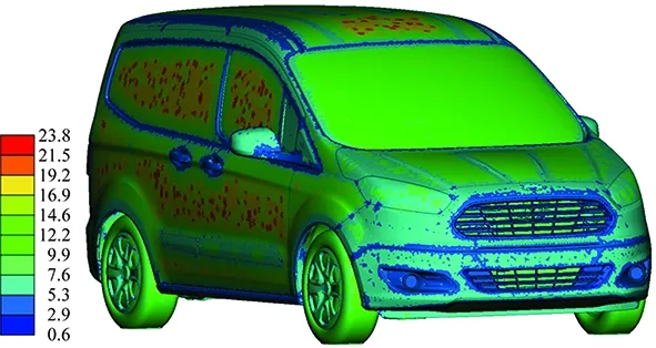
Fig. 1 Surface element lengths on the vehicle (mm).

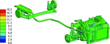
Fig.2 Surface element lengths at underbody components (mm).

Smaller element sizes were used on the surface of the vehicle at possible flow separation areas, stagnation regions and areas where a proper representation of geometry is needed. The mesh refinement is not performed only at the boundary layer development regions, but also in the wake regions. This grid structure is especially focused on the critical zones where sudden and significant changes occur in the flow properties. This ensures reliable results with lower computational time since the mesh refinement is only carried out at necessary locations. The local resolution of the surface and volume mesh elements can be increased by using the “size-box” property of ANSA grid generation software.ANSA size-boxes help to refine certain areas of surface and volume meshes without creating geometrical constructions for closed inner volumes [4].

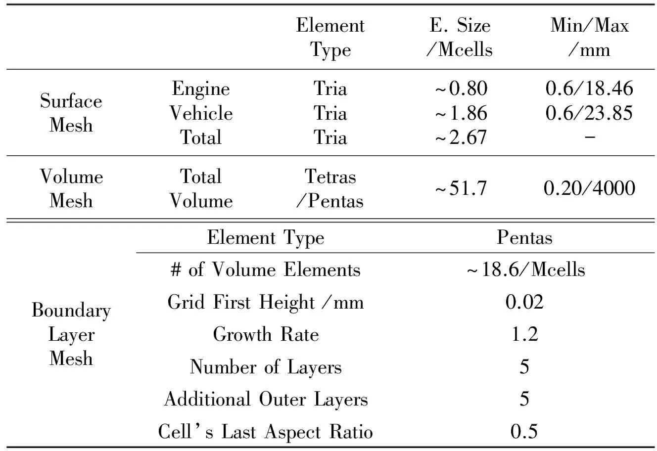
Table 2 Mesh specifications of the cooling drag analyses (open grill condition, Mcells: million cells)

The domain consists of approximately 51.7 million volume elements where almost one third of it comes from boundary layer region. Viscous sublayer length scale at the wall-adjacent cell should be on the order ofy+=1 when the enhanced wall treatment is employed with the intention of resolving the laminar sublayer [3]. The generated boundary layer and volume mesh specifications are given in Table 2 and shown in Fig. 3.

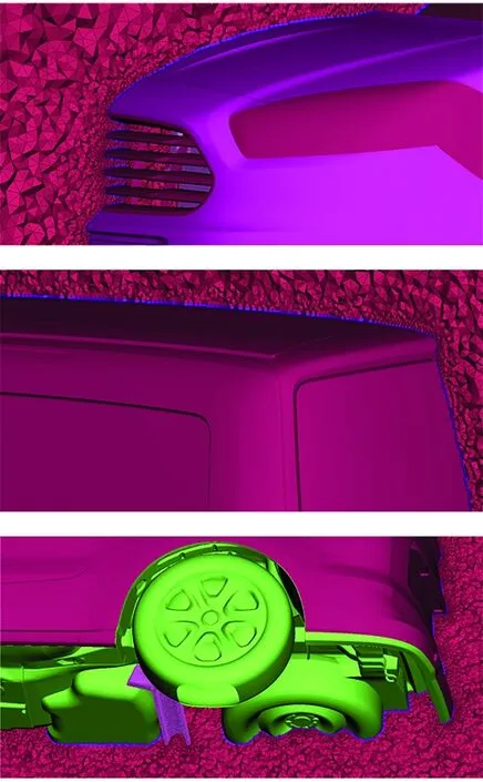
Fig.3 Boundary layer and volume mesh details.

1.4 Radiator and Fan Modeling

In CFD analyses, the radiator is generally treated as a porous medium or a heat exchanger that generates pressure drop. The pressure drop and heat transfer coefficient can be defined as a function of the perpendicular velocity component of the flow that passes through the radiator. It is assumed that the radiator element has a thickness which is infinitely thin and the pressure loss across the radiator is proportional to the dynamic pressure of the fluid. Experimentally determined dimensionless loss factors (kL) can be specified as constants or defined by polynomials and used as inputs for CFD analyses. The relation between dimensionless loss factor and pressure drop can be written as,

(1)

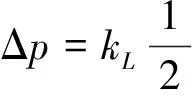
(2)

InEquations(1)and(2),ρis the density of the fluid (air),rnis the coefficients of the polynomial andvis the perpendicular velocity component of the flow passing through the radiator. In the present study, the heat exchanger model was assumed to have a pressure drop caused by radiator. The temperature change in cooling fluid was not taken into account. In experiments, the tunnel speeds ranging from 1.5 to 7.5 m/s were used deriving by the manufacturer data (e.g. mass-flow rate information of radiator fan). These speeds are also consistent with the reference studies found in literature [5,6]. The curve fitting is made to the measurements and given in Fig.4.

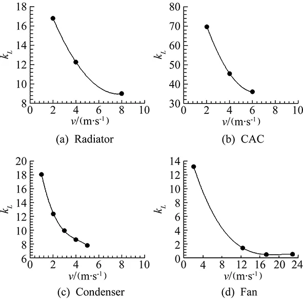
Fig.4 Fitted curves to loss measurements for the cooling system elements.

Numerical analyses is carried out to determine the cooling drag by implementing radiator definitions at relevant regions, Fig.5. Radiator definitions depend on polynomial expressions which were extracted from experiments.

The velocity distributions on the cooling components which are defined as radiator are presented in Figs. 6-8. The flow structures on the sections can be understood by examining the velocity component distributions. The CFD analyses show that the flow through the grills cannot form a homogeneous velocity distribution on the cooling sections. Moreover, remarkable change in velocity is observed especially in the directions which are tangent and perpendicular to the freestream direction.

Fig.5 Surfaces defined as radiators.

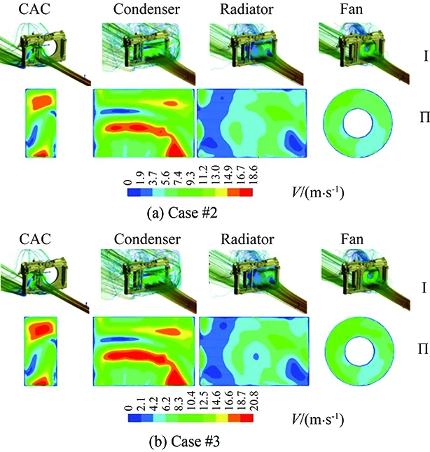
(Ⅰ) The streamlines and contours coloured by global velocity magnitudes (Ⅱ) The global velocity magnitudes at radiator surfaces Fig.6 Flow patterns and velocity field of the cooling components.

Fig.7 Local velocity distributions of the cooling components (Case#2).

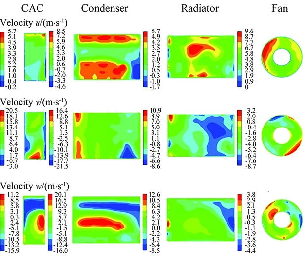
Fig.8 Local velocity distributions of the cooling components (Case#3).

In order to determine the cooling drag, additional cross-sections were constructed at the front and rear sides of the cooling components. As shown in Fig.9, the locations of these sections are at a distance of about 1 cm to the relevant surfaces.

The static pressure distributions at these surfaces are given in Figs.10-13. The area-weighted average of the static pressure values on the auxiliary sections were calculated to obtain the pressure drops.

The predicted pressure drop values are in a good agreement with experiments. The drag force due to the cooling system is calculated by multiplying the predicted pressure drops with the corresponding surface area. The total drag force is then obtained by summing the drag forces acting on the vehicle surface and the cooling components. The calculation is done by the following formulation:

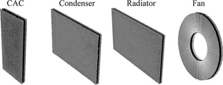
Fig.9 Cooling components (black) and the auxiliary surfaces (grey).

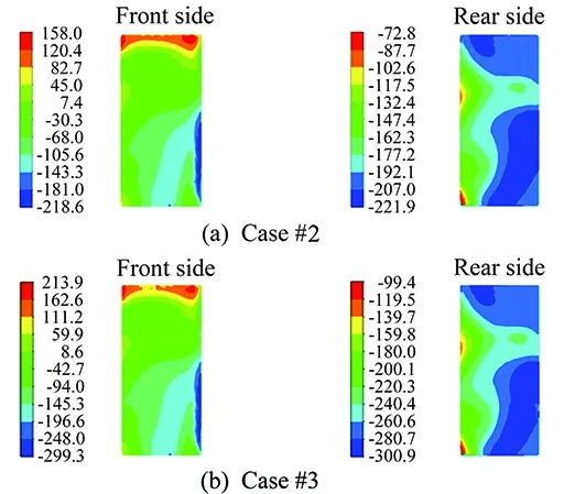
Fig.10 Static pressure distributions at auxiliary surfaces of CAC (Pa).

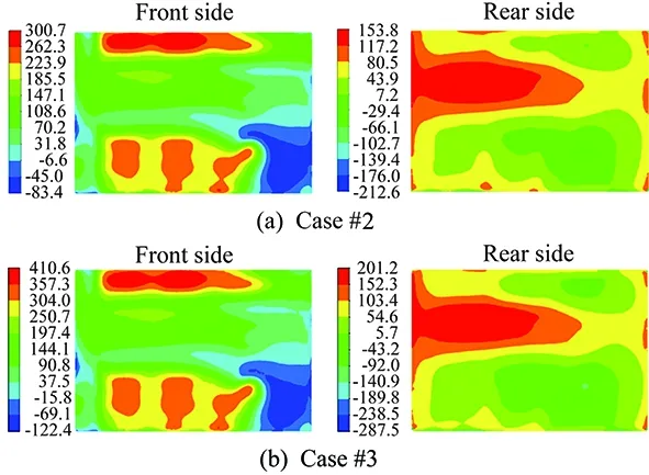
Fig.11 Static pressure distributions at auxiliary surfaces of condenser (Pa).

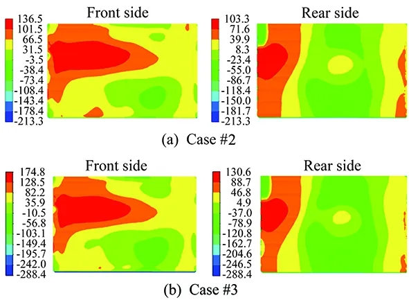
Fig.12 Static pressure distributions at auxiliary surfaces of radiator (Pa).

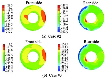
Fig.13 Static pressure distributions at auxiliary surfaces of fan (Pa).

FCS,i=ΔPCS,iACS,i

(3)

(4)

Inaboveequations,FVSis the net force acting on the vehicle surface andAVSis the frontal area of the vehicle.FCSis the net force acting on the cooling components obtained by the pressure drop values. Here,iis the index used for presenting each component of the cooling system. Therefore,ACS,iis the surface area of the relevant cooling component,qis the dynamic pressure and equals to 1/2ρU2for incompressible flows;ρis the mass density of the fluid (air) andUis the freestream velocity.

1.5 Results and Discussion

Case#1 and Case#2 were used to determine the drag caused by the cooling system. Results show that, the drag coefficient is increased by the implementation of cooling systems in the numerical model.

The effect of cruise speed on the prediction of drag coefficient was investigated via comparison of Case#2 and Case#3. The drag coefficient,CD, can often be treated as a constant for high Reynolds number flow regimes such as cars at highway speed or aircrafts at cruising speed. As shown in Fig. 10 to Fig.13, the predicted pressure distributions on the cooling components were qualitatively similar (almost identical) for the two cases but a quantitative examinaation shows that there exist differences in terms of pressure drops. In fact, it is observed that the drag force acting on the vehicle and cooling components become larger with the increased cruising speed, but the drag coefficient remained unchanged since the force is being made dimensionless with the square of the speed.

The effect of moving road and rotating wheels is also examined via comparison of Case#3 and Case#4. The resulting velocity contours for the flow field is presented in Fig. 14.

The flow velocity behind the wheels that are modeled as rotating walls is faster compared to the non-rotating ones. The rotating wheel model has also smaller wake compared to stationary one which yielded a lowerCDprediction. The predicted total drag coefficients of the aforementioned cases were tabulated with detailed descriptions in Table 3.

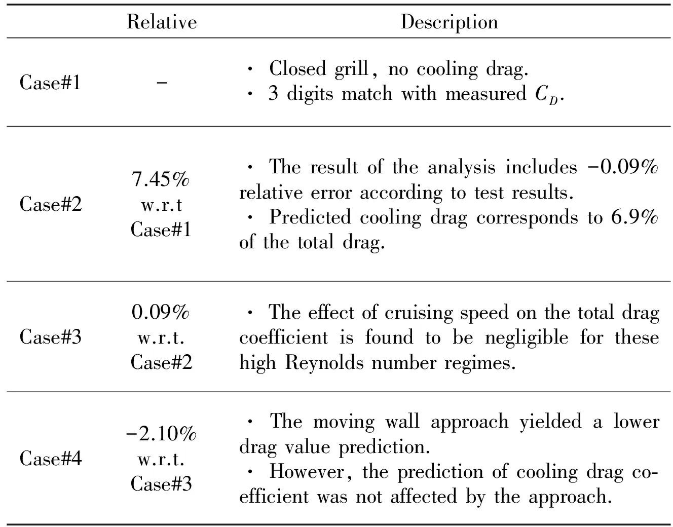
Table 3 Comparison of the total drag coefficients

The convergence histories of the different cases based on drag coefficient are given in Figs.15-17. The pressure coefficient distributions and the flow characteristics around the vehicle are shown in Fig.18 and Fig.19, respectively.

The geometric specifications of the vehicle and the drag coefficient values are not explicitly given due to commercial confidentiality.

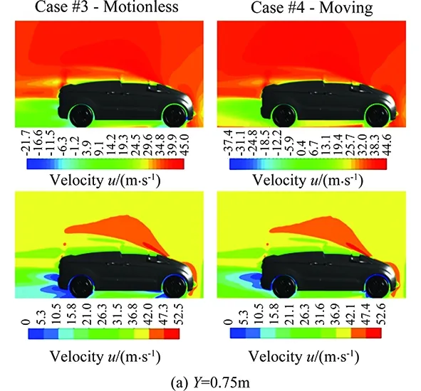
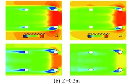
Fig.14 Effect of wheel motions on the velocity field predictions.

Fig.15 Effect of cooling drag on total CD.

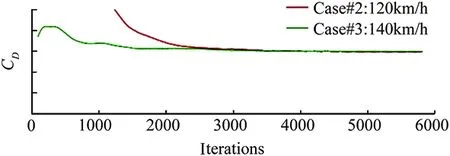
Fig.16 Effect of cruising speed on total CD.

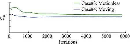
Fig. 17 Effect of moving road and wheel simulation on total CD.

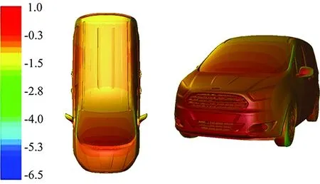
Fig.18 Cp distributions on the vehicle (Case#2).

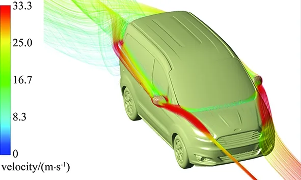
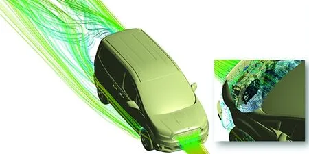
Fig.19 Flow characteristics for the cooling drag analyses (Case#2).

All calculations are carried out on a 12 core parallel machine with 2×2.30 GHz Intel Xeon E5-2630 pro-cessors. The platform uses a 64-bit Win-7 operating system and a total of 64 GB of RAM. The mesh partitioning is done using the “Metis” method of the FLUENT software. The wall clock computation time was approximately 114.5 h for a solution of 6000 iterations. It is observed that the radiator/fan modeling and the moving wall approach do not have a noticeable effect on the computation time.

2 Conclusions and Future Work

CFD analyses have been performed to obtain total drag coefficient including cooling drag part for the light commercial vehicle. The pressure drop characteristics of the cooling system components are determined by wind tunnel tests utilizing the facilities of ITU Trisonic Laboratory and manufacturer's data provided by FORD. ITU wind tunnel tests have been carried out by additional studies to validate the manufacturer’s data and examine the various working-conditions (free and force-fed) of fan.

CFD analysis results are consistent with the clay model test results. A satisfactory result gathered from CFD analysis (Case#2) with a 0.1% approxi-mation to the clay model test results.

The CFD analysis for the closed grill condition represented by Case#1 have been made to isolate the effect of cooling drag on the total drag. Predicted cooling drag corresponds to 6.9% of the total drag which is consistent with the test results

and measurements by the manufacturer. Furthermore, additional analysis for different cruising speeds such as 120 km/h and 140 km/h demonstrated that the cruise speed, particularly for these flow regimes, do not have a remarkable effect on the prediction of cooling drag coefficient. Likewise, the prediction of cooling drag coefficient does not change whether the CFD model includes the road and wheel motion. However, modeling the road and wheel motion reduces the total drag coefficient.

The cooling drag characteristics of different vehicles can be determined by using the modeling methodology developed in the present work. The cooling flow may be obtained with lower pressure loss by the optimization studies to be performed on the vehicle.

[1] Anbarci K, Acikgoz M B, Aslan A R, et al. Development of an aerodynamic analysis methodology for tractor-trailer class heavy commercial vehicles[J]. SAE Int. J. Commer. Veh. , 2013, 6(2):441-452.

[2] D’Hondt M, Gilliéron P, Devinant P. Flow in the engine compartment: analysis and optimization[J]. International Journal of Aerodynamics, 2011, 1, 3/4, 384- 403.

[3] FLUENT Inc, 2013.

[4] BETA CAE Systems ANSA Version 13 User Manual[M/OL]. www.beta-cae.gr.

[5] Ngy Srun Ap, Pascal Guerrero, Philippe Jouanny. Influence of front end vehicle, fan and shroud on the heat performance of A/C condenser and cooling radiator[R]. SAE Technical Paper Series, 2002-01-1206, 2002.

[6] Berg T, Wikstrom A. Fan modelling for front end cooling with CFD[D]. Sweden: Volvo Cars and Lulea University of Technology, Masters Thesis.2007.

0258-1825(2016)02-0232-07

冷却系统阻力对汽车总阻力影响的数值预测模型研究

A. Rustem Aslan1,*, Kerem Anbarci2, M. Berkay Acikgoz2, Omur Icke3, Ozgur Aslan3, Cenk Dinc3

(1. Istanbul Technical University, Maslak, Istanbul 34469, Turkey; 2. AES-Aero Engineering Ltd., Turkey; 3. FORD Motor Company, Turkey)

采用CFD方法数值模拟了小型汽车发动机冷却系统对全车阻力的影响特性。汽车的内部及外部(发动机舱及舱内)均设置了数值模拟网格。分别计算了散热器及风扇对阻力的影响，采用本校实验结果(散热器压力损失)及制造商提供的数据(散热器及风扇的质量流率)确定初始及边界条件，为基于RNS的CFD提供输入。对汽车轮胎运动模式及行驶速度对散热系统阻力及汽车总阻的影响特性也进行了计算分析。预测结果表明，冷却系统阻力占汽车总阻的6.9%，与实测值吻合。

数值方法；计算流体力学；湍流模型；冷却系统阻力；散热器；风扇；实验测量

V211.3

A doi: 10.7638/kqdlxxb-2016.0012

*Professor, Department of Aerospace Engineering; aslanr@itu.edu.tr

format: Aslan A R, Anbarci K, Acikgoz M B, et al. Numerical Modeling and Prediction of the effect of cooling drag on the total vehicle drag[J]. Acta Aerodynamica Sinica, 2016, 34(2): 232-238.

10.7638/kqdlxxb-2016.0012. Aslan A R, Anbarci K, Acikgoz M B, 等. 冷却系统阻力对汽车总阻力影响的数值预测模型研究(英文)[J]. 空气动力学学报, 2016, 34(2): 232-238.

Received date： 2016-02-04; Revised date: 2016-03-18