
Calculation of tip vortex cavitation flows around three-dimensional hydrofoils and propellers using a nonlinear k -ε turbulence model*
2016-10-14 12:23ZhihuiLIU刘志辉BenlongWANG王本龙XiaoxingPENG彭晓星DengchengLIU刘登成
水动力学研究与进展 B辑 2016年2期
Zhi-hui LIU (刘志辉),Ben-long WANG (王本龙),Xiao-xing PENG (彭晓星),Deng-cheng LIU (刘登成)
1.Department of Engineering Mechanics and Key Laboratory of Hydrodynamics of Ministry of Education,Shanghai Jiao Tong University,Shanghai 200240,China,E-mail:lzh119160@163.com
2.China Ship Scientific Research Center,Wuxi 214082,China
Calculation of tip vortex cavitation flows around three-dimensional hydrofoils and propellers using a nonlinear k -ε turbulence model*
Zhi-hui LIU (刘志辉)1,Ben-long WANG (王本龙)1,Xiao-xing PENG (彭晓星)2,Deng-cheng LIU (刘登成)2
1.Department of Engineering Mechanics and Key Laboratory of Hydrodynamics of Ministry of Education,Shanghai Jiao Tong University,Shanghai 200240,China,E-mail:lzh119160@163.com
2.China Ship Scientific Research Center,Wuxi 214082,China
Simulations of tip vortex wetted flows and cavitating flows are carried out by using a RANS model.Two types of turbulence models,with and without the Boussinesq turbulent-viscosity hypothesis,are adopted in comparing with experimental results regarding the vorticity,the strain rate and the Reynolds shear stress distributions in the vortex region.The numerical results imply that the spatial phase shift between the mean strain rate and the Reynolds stresses can be accurately modeled by the nonlinear k-ε turbulence model,the tip vortex cavitation region can only be predicted using the nonlinear k-ε turbulence model.The mechanism of the over-dissipation due to the turbulence model is analyzed in terms of the turbulence production,which is one of the dominant source terms in the transport equations of energy.
tip vortex,tip vortex cavitation,Boussinesq turbulence viscosity model,nonlinear turbulence model,Open FOAM
Introduction
Tip vortex flows are found in various situations,including those around air foils,helicopter blades,wind turbines,hydrofoils and marine propellers.In the marine engineering,the tip vortex flows also accompany the tip vortex cavitation due to the large tangential velocity and pressure drops.The tip vortex cavitation results in vibrations and cavitation erosions of propellers and rudders,particularly for high-speed ships.The experimentation has been the primary tool for studying the formation and the flow characteristics of the tip vortex cavitation of hydrofoils and propellers over a long time[1].Measurements of the tip vortex flows are usually difficult and time-consuming.Dueto the interface between the liquid and the vapor phases,detailed optical observations of the cavitating flow field inside the vortex region are very difficult,using advanced computational fluid dynamics to accurately predict the tip vortex flows is not simple but is possible.The most challenging task is to properly simulate the tip vortex cavitation.
Although the detached eddy simulations and the large eddy simulation have been successfully applied for cavitating flows[2,3],the Reynolds averaged Navier-Stokes equations remain the primary CFD solver used in practical applications due to their low computational cost.However,the widely used two-equation turbulence models perform poorly for highly rotational flows.The intrinsic assumption of the Boussinesq turbulent-viscosity hypotheses,which states that the shear stress is locally determined by the mean strain rate,has no general validity[4].
Chow et al.[5]measured the distribution of the strain rate and the Reynolds shear stresses in the tip vortex region.It is found that the four-leaf clover pattern of these two contours is not aligned spatially,indicating that the flow is not isotropic.We denote this type of rotation as a spatial phase shift in the present work.Similar experimental results for flows atdifferent angles of attack and Reynolds numbers were obtained recently by Giuni[6].The Boussinesq turbulent-viscosity hypothesis assumes that the Reynolds shear stresses depend linearly on the shear strains.These detailed experimental data imply that the turbulence models based on the Boussinesq turbulent-viscosity hypothesis are not capable of describing the vortex evolution in the near wake of hydrofoils and propellers.Churchfield and Blaisdell[7]explored several turbulence models and corrections for system rotation and streamline curvature,including a one-equation model,two-equation models and a shear stress transport model.It is found that none of these turbulence models can accurately capture the spatial lag between the Reynolds stress components and the corresponding strain rate components within the vortex.
Using two-equation turbulence models under the Boussinesq hypothesis,the sheet cavitations on the blade and the hydrodynamic loading can be accurately predicted,as reported by Liu et al.[8]and Zhu and Fang[9]using an RNG k-εmodel and by Yang et al.[10]using thek-ωmodel.However,these models could not correctly capture the cavitating tip vortex.On the other hand,an explicit algebraic Reynolds stress model was successfully used to simulate the tip vortex cavitation flow around an elliptical hydrofoil[11].Good agreement with experimental results was obtained for the desinence cavitation number and the cavitating tip vortex.
To correctly predict the vortex cavitating flows,the performance of the turbulent models without the Boussinesq hypothesis is studied in this paper.The standard k-εmodel and the nonlinear k-εturbulence models are compared with experimental data.Then the tip vortex cavitating flows near a propeller blade are investigated.
1.Numerical models
1.1 Governing flow equations
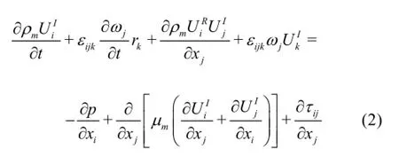
To simulate the cavitating flow around airfoils or propellers,the assumption of a homogeneous mixed fluid of water and vapor is adopted,the liquid and vapor phases are assumed to be fully mixed and share the same velocity and pressure in the flow field.The turbulent viscous flows are solved using the Reynolds averaged Navier-Stokes equations.Specifically,there are two regions in the computational domain:the internal region and the external region.In the internal region,a rotating reference frame is employed to simulate the flows around the propeller,where the RANS equations are:
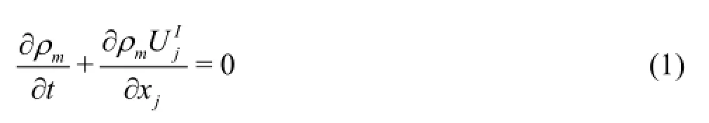
In the external region,the typical RANS equations in static coordinates are solved as
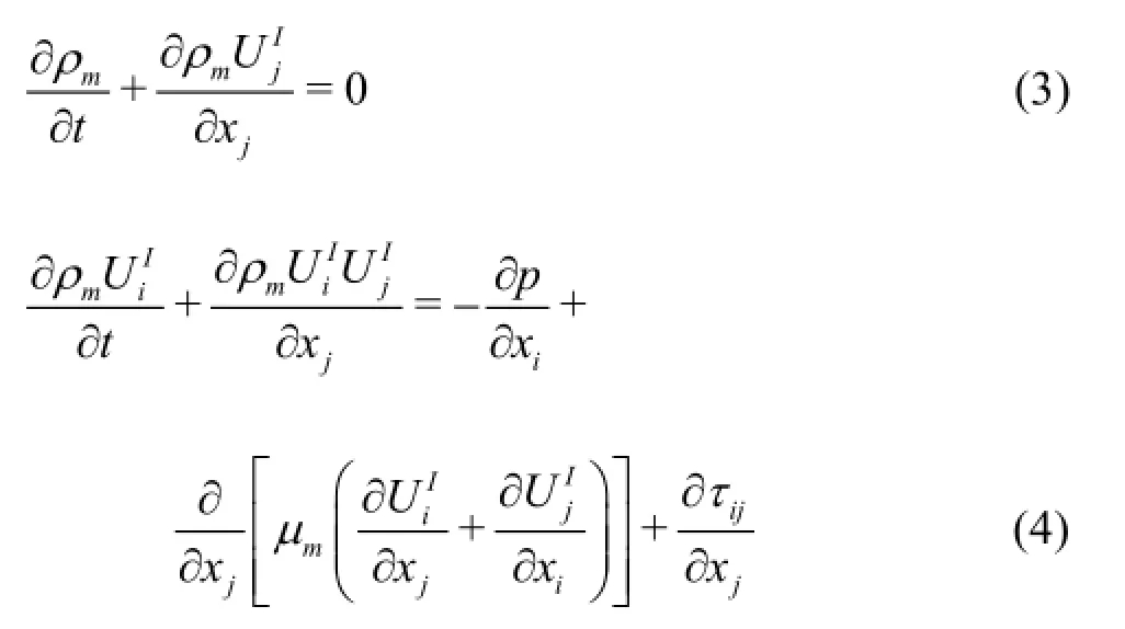
where xiand tare the spatial coordinates and the time,respectively,pis the pressure,andandare the Reynolds averaged velocities.The superscripts of I and R represent the absolute and relative velocity components in the rotating frame,respectively.The relationship betweenandisis the angular velocity of the rotating frame andriis the rotating radius.ρmand µmare the average density and the molecule viscous coefficient of the water and vapor mixture,respectively,αland αvare the volume fractions of the liquid phase and the vapor phase in each computational cells,respectively,τi jis the Reynolds stress due to the fluctuating velocity field.To close the flow equations,turbulence models are required to calculate the Reynolds stress τij.
1.2 Standard k-ε model
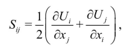
The Boussinesq turbulent-viscosity hypothesis has been used successfully in many turbulence flows.One type of closure model is the standard k-εturbulence model,which will be examined first.Under the Boussinesq assumption,the deviatoric Reynolds stress part (or Reynolds shear stress)is linearly proportional to the mean rate of strain:
where µtis the turbulent viscosity (i.e.,the eddy viscosity),δijis the Kronecker delta,andkis the turbulent kinetic energy.The turbulent viscosity can be calculated asµtin the standard k-εturbulence model[16]with Cµ=0.09 and a turbulent kinetic dissipation rate expressed as
1.3 Nonlinear k-εmodel
The Boussinesq turbulent-viscosity hypothesis was proposed initially for pure shear flows.As a result,the orientations of the strain rate tensor and the Reynolds stress tensor are assumed to coincide.However,this type of linear models fail when the flow stream is curved or strongly rotated[12].Experimental observations show that the strain rate and the Reynolds stress are not aligned in their tip vortex region[5,6].Thus,a nonlinear k-εmodel is employed in the present study.Note that the nonlineark-εmodel is not a simple extension of the standardk-εmodel.Essentially,the Boussinesq turbulent-viscosity hypothesis is discarded in the nonlineark-εmodel.The nonlinear relationship between the Reynolds shear stress and the strain rate satisfies the non-isotropic constitutive relation by summation of the strain rate tensor and the rotation rate tensor[4].
Although the theoretical foundation of the nonlinear k-εmodel is significantly different from that of the standardk-εmodel,the numerical implementation is straightforward by extension of the standard k-εmodel.The relationship between the shear stress and the strain rate is
where

In this turbulence model,the rotation rate is also included in the constitutive relationship.The nonlinear k-εmodel is a high-Reynolds-number model with wall functions,denoted as Nonlinear KEShih in Open FOAM,which is also known as the realizable Reynolds stress algebraic equation model.The rotational effect of the mean flow is described byCd.
1.4 Cavitation model
The phase transition strongly depends on the saturation pressure of the water vapor and other factors,pv=2300 Pais assumed in the present work.To simulate the phase transition between the liquid and vapor phases,a cavitation model is needed.The transport equation model has been widely used in recent numerical studies of cavitating flows.Examples of such models were given by Schnerr and Sauer[13],Singhal et al.[14]and Zawart et al.[15].These types of cavitation models have been successfully used in simulations of various unsteady cavitating flows.The transport equation of Schnerr and Sauer is used in the present work.
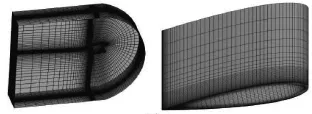
Fig.1 Illustration of mesh in the computational domain and on the surface of a hydrofoil
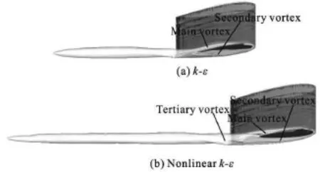
Fig.2 Iso-surface with Q =103,at the same mesh resolution
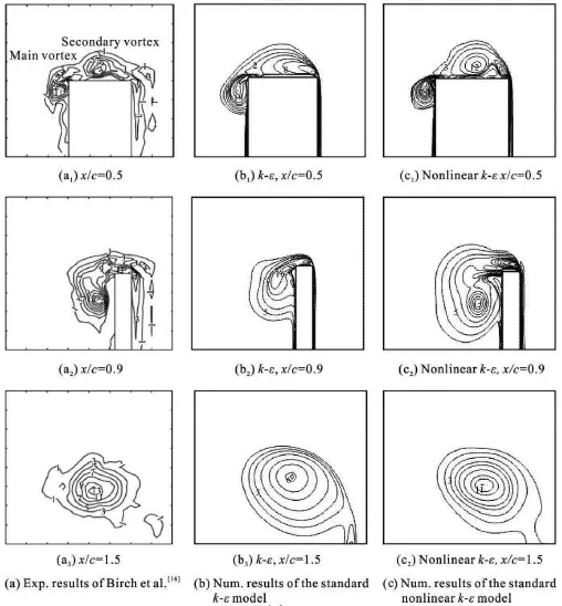
Fig.3 Distributions of dimensionless vortex contours at different locations
2.Numerical method and implementations
The numerical models detailed in the previous section are solved by using a finite volume method based on the OpenFOAM package.The PISO scheme is used to solve for the velocity/pressure coupling between the momentum and continuity equations.A second-order upwind scheme is used for the spatial discretization in the momentum and transport equations forkandε.The QUICK scheme is used in the advection of the volume fraction function.The viscous terms are solved using a second-order central difference scheme.
Four types of boundaries are used:(1) the upstream inlet boundary condition,where the velocity is specified and the values of the VOF function are set to αv=0,(2) the outlet boundary condition or the downstream far field condition,where the pressure is prescribed according the cavitation number and the normal gradient of the velocity and other scalar functions are set to zero,(3) the no slip boundary condition at a solid surface (e.g.,on airfoils,propeller blades),where the velocity components are all set to zero on the wall surface,and the normal gradient of the scalar function (e.g.,the pressure or the VOF function) is set to zero,(4) the symmetry conditions,where no material flux across the symmetry boundary,and thus the gradient of the normal velocity and the normal gradient of the scalar functions (e.g.,the pressure or the density) are set to zero.
The boundary conditions forkand ε are specified at the inlet:,which are also given as the initial conditions in the computational domain.U is the incoming velocity,I=0.05 is the turbulence intensity,and l is the characteristic length,or the chord length for hydrofoils and the diameter for propellers.
3.Tip vortex flows of a three dimensional hydrofoil
Although the elliptical foils or propellers are common underwater structures,the tip vortices around a truncated plane airfoil can provide significant information without the interference of other complex flows.To study the details of the turbulent flows,we focus on the vorticity,the strain rate and the Reynolds stress distributions instead of the integration quantities,such as the hydrodynamic loads,in the present work.
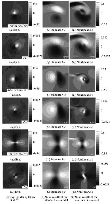
Fig.4 Comparison of spatial distribution of negative strain rate and deviatoric Reynolds stress between experiment results and numerical simulations:NACA0015,attack angle α=10o,Re=4.6× 10⁶,x=1.452C .(XV,YV)=(0,0)is the center of the vortex
3.1 Structure of tip vortex
First,we study the tip vortices around a rectangular,square-tipped NACA0015 hydrofoil,which is the most simple tip vortex flow and can reflect the flow structure in a straightforward way.The three-dimensional flow structures of a tip vortex in the near wake of a rectangular,square-tipped NACA0015 airfoil were measured using a seven-hole pressure probe atRe=2.01× 10⁵[16].The ratio of the span to the chord length is 1.5.In this subsection,we compare the numerical results with experimental data for the vortex strength and structure in the near wake region.The mesh convergence test is conducted for the drag and lift6force.The final mesh includes approximately 1.2× 10 computational cells,as shown in Fig.1.The local adaptive mesh refinement is applied in the tip region.
At the same mesh resolution,the computational results are shown in Fig.2 for a value of Q,which identifies the vortex structures in the turbulence flow.The range of the is o-surface of Q extends much more farther in the nonlinear k-ε turbulence model than in the standard k-εmodel.The tertiary vortex could be captured in the simulation with the nonlinear k-ε turbulence model.
Figure 3 shows the representative normalized streamwise vorticity contour of the tip vortex,i.e.,Ω11C/2U∞,at different locations of x=0.5C,0.9C and1.5C ,in which U∞is the streamwise velocity,Ω11is the strength of the rotation rate,and Cis the chord length.The planes x =0and x=Care the sides cutting the leading edge and the trailing edge of the hydrofoil.Three vortex structures are well captured by the nonlineark-εturbulence model at the locations around the foil (i.e.,0.5C≤x≤0.9C).During the evolution of the three vortexes further downstream,as shown in Figs.2 and 3,a single vortex is formed by the convergence of the other two at x= 1.5C.However,only a primary vortex and a secondary vortex can be resolved by the standard k-εturbulence model.
3.2 Spatial distribution of strain rate and Reynolds stress
The measurements of the tip vortex flow at various attach angles (4o-12o)and Reynolds numbers (5× 10⁵-4.6× 10⁶) were conducted[5,6].Four-lobe patterns were found for both the strain rate and the Reynolds stress in these experimental results.All experimental results show that there is a spatial phase shift of the four-lobe pattern between the strain rate and the Reynolds stress,as shown in Fig.4(a):a phase shift ofπ/4can be observed between the strain rates εxy,εyzand the corresponding components of the Reynolds stress,and a phase shift ofπ/2can also be observed between the strain rateεxzand the Reynolds stress
For a rounded wingtip NACA0012 hydrofoil,the numerical simulation is conducted to study the spatial distribution of the strains and the Reynolds stresses.The Reynolds number is Re=4.6× 10⁶,and the angle of attack is α=10o.The computational mesh is similar to that in Fig.1 except the rounded wingtip geometry is used.The numb6er of the total mesh cells is approximately 4.5×10 due to the high Reynolds number.
If the eddy viscosity remains constant in the core region of the vortex,this type of phase shift indicates that the linear relationship between the strain rate and the Reynolds stress does not hold.The Boussinesq turbulent-viscosity hypothesis in Eq.(5) is not suitable for the tip vortex turbulence flow[17].In fact,the Boussinesq turbulent-viscosity hypothesis is based on the pure shear turbulence flows,thus,the Reynolds stress depends only on the strain rate Sij.For the tip vortex flow,the contribution of the rotation rateΩijis significant but absent in Eq.(5).These experimental observations show why non-Boussinesq turbulence models have to be used to describe the tip vortex flows.
The numerical results of two different turbulence models are given in Figs.4(b) and 4(c).The numerical results of the standard k-εmodel shows that the distributions of the strain rate and the Reynolds stress are in the same four-lobe pattern,which is a consequence of the linear relationship between the strain rate and the Reynolds stress under the Boussinesq turbulent-viscosity hypothesis.On the other hand,the numerical results of the nonlinear k-εmodel show a significant improvement in the spatial distributions of the Reynolds stress,particularly in the components of
3.3 Turbulence production and analysis of energy dissipation
Numerical results of both the vortex structure and the distribution of the stain rate and the Reynolds stress verify the advantages of the nonlinear k-ε model in the numerical simulations of the tip vortex flows.The advantages of this model can be explained from the perspective of an energy budget.Defining the kinetic energy of the mean flowto be E=UiUi/2 and the turbulent kinetic energy to bek ,the transport equations of these two types of energy are:
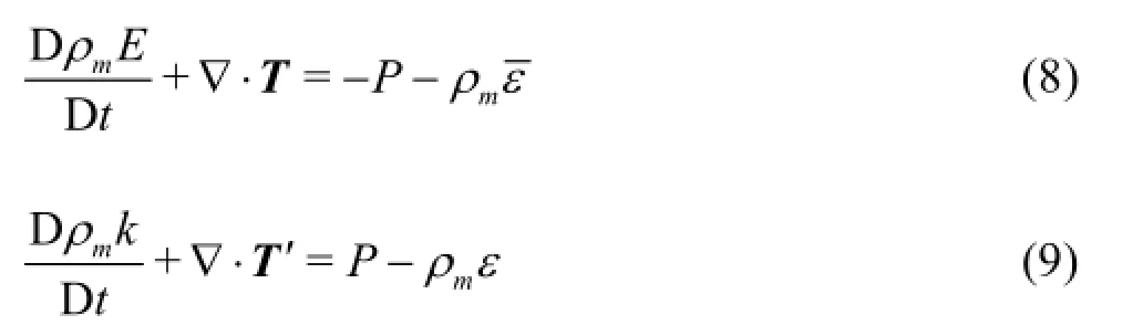
whereD/Dt is the total derivative,is the viscous dissipation rate of the mean flow stain rate due to the molecule viscosity,ρmεis the turbulent kineticdissipation rate,related with the strain rate of the fluctuate velocity field,Tand T′are the convections of the Reynolds stress,the pressure stress and the molecule viscosity by the mean and fluctuated velocities,respectively[4],and T′is modeled by (µm+µt/ σk)∂k/∂xjin the standard k-ε model.
Recalling the definition of the production P=due to the fact that the turbulent eddy viscosity is much larger than the molecular viscosity µt≫µm.Therefore,the primary source in the right hand side of Eq.(8) is contributed by the production term P.The production Pextracts the total kinetic energy from the mean flow and transfers it to the turbulent kinetic energy.The production Pthus serves as a sink term in Eq.(8) and a source term in Eq.(9).The correct prediction of the magnitude of the production Pinfluences the energy transfer between the mean and fluctuating flows.Finally,the amount of the transfer energy is dissipated at the turbulent kinetic dissipation rate ρmε.For homogeneous and steady turbulent flows,we haveP≈ε.Therefore,the turbulent dissipation may be estimated by the magnitude of the productionP.IfP is over-estimated,the strength of the vortex will be under-estimated.
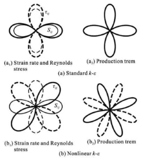
Fig.5 Effects of phase shift on the production term.Positive value is shown in solid lines and negative value in dashed lines
To illustrate the effects of the phase shift on the production term,a typical four-lobe distribution of the strain rate and the Reynolds stress components is plotted at a prescribed circle around the vortex center in Fig.5.For turbulence models based on the Boussinesq hypothesis,the strain rate and the Reynolds stress have the same sign along the circle and thus a maximum production termis obtained.In the nonlinear k-εmodel,there is a phase shift between the strain rate and the Reynolds stress,as observed experimentally[9,10].Thus the integration ofover the cross-section will be partially canceled.Therefore,the nonlinear k-ε model must have less production (i.e.,turbulence dissipation) than the standard k-ε model.
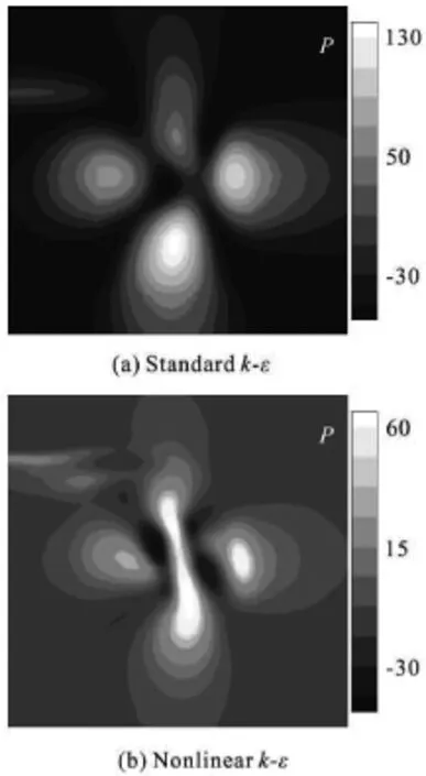
Fig.6 Distribution of production term at x=1.452C
The numerical integration of Pat x=1.452C can now be compared between the two turbulence models.Expanding the production term yields
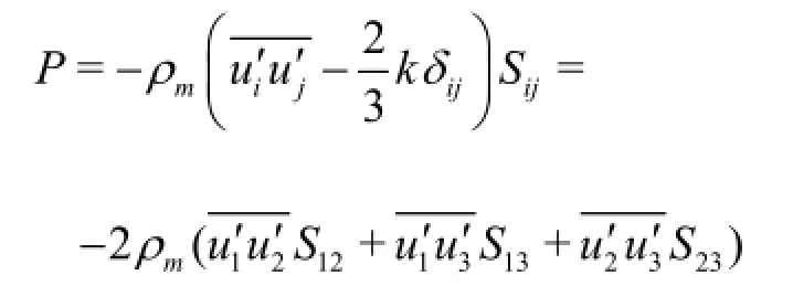
The magnitude of the production integral Et=predicted by the nonlinear k-ε model is 2.83 at x=1.452C,much smaller than that of the standard k-ε model,which is 4.08,as shown in Fig.6.This conclusion can be easily obtained by a direct comparison of the distribution of the strain rate and the Reynolds stress shown in Fig.4.For the numerical results of the standard k-ε model,there is no phase shift of the four-lobe pattern; the productions of the strain rateandthus reach the maximum valuesin each lobe.Once there is a phase shift,as shown in the experimental results and the numerical results of the nonlinear k-ε model,the integration will be partially cancelled,while the production calculated under the Boussinesq turbulent-viscosity hypothesis is at its maximum,i.e.,the linear turbulence model introduces a significant turbulent dissipation.To capture the spatial phase shift can be taken as a pre-requirement of the success of the tip vortex simulation.
4.Tip vortex and tip vortex cavitation of propellers
The numerical simulations of the tip vortex flows around a three-dimensional hydrofoil verify the present flow solver.In this study,the INSEAN E779A four-blade propeller with a diameter D=0.227 m,the nominal pitch ratio 1.1,the hub diameter 0.0453 m is examined.The incoming velocity isU∞=5.808 m/s,and the advance ratioJ=U/ nD=0.71.The cavitation number is σn=(P-Pv)/2(n D)2=1.763in the following analysis.The full structural meshes are used in these simulations.The total number of computational cells is approximately 4.5×10⁶after the Oct-tree refinement in the wake region of the propeller tip,the selected meshes are shown in Fig.7.
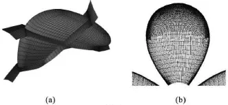
Fig.7 Local refinement of meshes on surface of one propeller blade
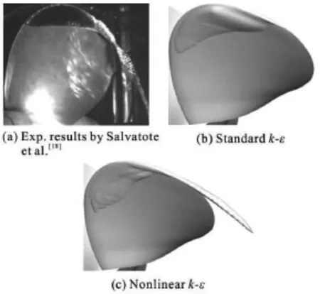
Fig.8 Comparison of the vapor volume fraction with αv=0.1
At the same mesh resolution,the regions of the sheet cavitation and the tip vortex cavitation are shown in Fig.8 for the two turbulence models.The cavitation regions are compared with the experimental results by Salvatore et al.[18].The areas of the sheet cavitation predicted by the numerical simulations are qualitatively similar on the surface of the blade,and both agree with the experimental results.The primary differences lie in the tip vortex cavitation,which can be predicted when the nonlinear k-ε model is employed.The tip vortex cavitation also depends on the mesh resolution in the vortex region.To capture the tip vortex cavitation zone better,the mesh refinement in the near wake is necessary.
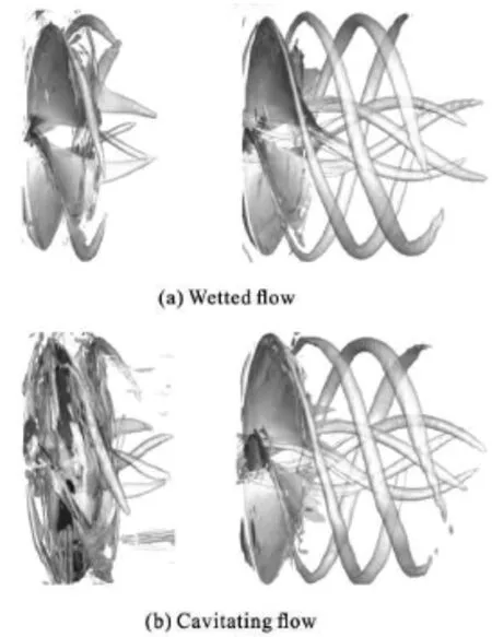
Fig.9 Iso-surface of Q =104at the same mesh resolution
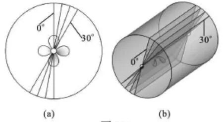
Fig.10 Definition of each plane
The iso-surface of the second invariance Qis shown in Fig.9 for wetted and cavitating flows.The tip vortex region is shown to be less dissipated by the turbulence as predicted by the nonlinear k-εmodel.When the tip vortex is less dissipated,the strength of the vortex can stretch over a longer distance,allowing the tip vortex cavitation region to be captured.
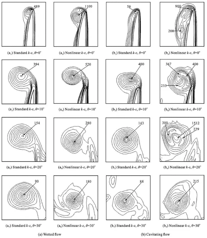
Fig.11 Distributions of dimensionless vorticity
To produce a more in-depth picture of the flow field,we define four planes,as shown in Fig.10.The plane of θ=0ocrosses the x-coordinate and the radius across the tip of one blade.The angle between the neighboring two planes is10o.We compare the dimensionless vorticity defined asand R=D /2.The distributions ofin each plane(x/ R,r/ R)are given in Fig.11 for wetted flow and cavitating flows.
For both wetted and cavitating flows,the magnitude of the vorticitypredicted by the nonlinear k-ε modelis nearly twice of that predicted by the standard k-ε model.The vortex center detaches from the blade surface,as shown in the plane with θ=0owhen the nonlinear k-ε model is used.Another difference is that the diameter of the vortex tube is small as predicted by the nonlinear k-ε model,which implies that the total circulation is kept nearlyconstant.
For cavitating flows,the numerical results obtained with the nonlinear k-εmodel show a multivortex structure in the wake region (e.g.,θ=10oand θ=20o) in contrast to the single vortex structure shown in wetted flows.Due to the generation of cavitation,there is a slight difference in the vortex strength between cavitating and the wetted flows.
Similar relationships between the strain rate and the Reynolds stress can be found in both wetted and cavitating flows in the propeller's tip vortex region.Significant differences of the tip vortex length,as shown in Fig.8,and the iso-surface of Q ,as shown in Fig.9,are related with the correct prediction of the vortex strength (i.e.,turbulent dissipation ε).Due to the phase shift of the spatial distribution of the strain rate and the Reynolds stress,the accuracy of the eddy viscous dissipation can be improved by using the nonlinear k-ε model.
For the turbulent flows around the propeller's blades,the vortex structure becomes more complex.However,the spatial distributions of the strain and the Reynolds stress show the same pattern in the numerical results with the standard k-ε model.When the nonlinear k-ε model is used,the spatial phase shift is predicted accurately.
The integration of the production term in the plane of θ=20ois shown in Table 1.For the propeller studied,the production is much smaller when predicted by the nonlinear k-ε model than when predicted by the standard k-ε model for both wetted and cavitating flows.
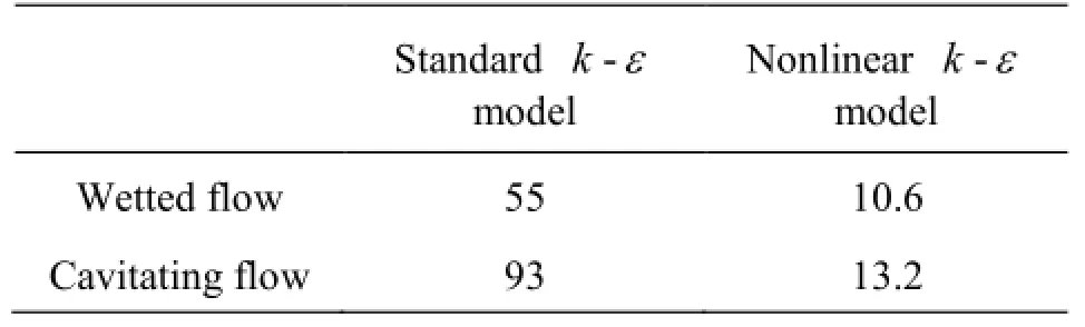
Table 1 Integral production term Et=∫∫Pds,θ=20o
The mesh resolution is also shown to affect the vortex wake,using a fine mesh can resolve tip vortices further downstream.Therefore,an adaptive mesh refinement in the vortex wake region is important to capture the detailed flow field away from the propeller.
5.Conclusions and remarks
Details of the turbulent flow fields in the tip vortex regions of three-dimensional hydrofoils and propellers are obtained by using two common turbulence models:the standard k-ε model and the nonlinear k-εmodel.The most fundamental difference between these two turbulence models is with or without the Boussinesq turbulent-viscosity hypothesis.In the tip vortex region,in both wetted and cavitating flows,a spatial phase shift of distribution can be reasonably predicted by the nonlinear k-εmodel,which agrees with experimental observations.The advantages of the nonlineark-εmodel include the fact that the rotation rate is also included in the constitutive relationship between the strain and the Reynolds stress,which implies that the correction of the rotating flow is important in the tip vortex simulations.
In the present work,investigations are performed in the same mesh for each case.In the mesh convergence tests,it is also found that the spatial distribution pattern would not change when finer resolutions are used.The numerical results shown in this paper imply that the nonlinear k-εmodel is a promising candidate for predicting the tip vortex cavitation flows in practical applications at a much lower computational cost compared to other advanced turbulence models,including the detached eddy simulations and the large eddy simulations.
[1]ARNDT R.E.A.,ARAKERI V.H.and HIGUCHI H.Some observations of tip-vortex cavitation[J].Journal of Fluid Mechanics,1991,229:269-289.
[2]WANG Ya-yun,WANG Ben-long and and LIU Hua.Numerical simulation of sheer cavity shedding and cloud cavitation on a 2D hydrofoil[J].Chinese Journal of Hydrodynamics,2014,29(2):175-182(in Chinese).
[3]ZHANG Ling-xin,ZHANG Na and PENG Xiao-xing et al.A review of studies of mechanism and prediction of tip vortex cavitation inception[J].Journal Hydrodynamics,2015,27(4):488-495.
[4]POPE S.B.Turbulent flows[M].Cambridge,UK:Cambridge University Press,2000,126,365.
[5]CHOW J.S.,ZILLIAC G.G.and BRADSHAW P.Mean and turbulence measurements in the near field of a wingtip vortex[J].AIAA Journal,1997,35(10):1561-1567.
[6]GIUNI M.Formation and early development of wingtip vortices[D].Doctoral Thesis,Glasgow,UK:University of Glasgow,2013.
[7]CHURCHFIELD M.J.,BLAISDELL G.A. Numerical simulations of a wingtip vortex in the near field[J].Journal of Aircraft,2009,46(1):230-243.
[8]LIU D.,HONG F.and ZHANG Z.et al.The CFD analysis of propeller sheet cavitation[C].8th International Conference on Hydrodynamics,Nantes,France,2008.
[9]ZHU Zhi-feng,FANG Shi-liang.Numerical investigation of cavitation performance of ship propellers[J].Journal Hydrodynamics,2012,24(3):347-353.
[10]YANG Qiong-fang,WANG Yong-sheng and ZHANG Zhi-hong.Assessment of the improved cavitation model and modified turbulence model for ship propeller cavitation simulation[J].Journal of Mechanical Engineering,2012,48(9):178-185(in Chinese).
[11]HAN Bao-yu,XIONG Ying and LIU Zhi-hua.Numericalstudy of tip vortex cavitation using CFD method[J].Journal of Harbin Engineering University,2011,32(6):702-707(in Chinese).
[12]RUNG T.,THIELE F.and FU S.On the realizability of nonlinear stress-strain relationships for Reynolds stress closures[J].Flow,Turbulence and Combustion,1998,60(4):333-359.
[13]SCHNERR G.H.,SAUER J.Physical and numerical modeling of unsteady cavitation dynamics[C].Proceeding of the 4th International Conference on multiphase Flow.New Orleans,La,USA,2001.
[14]SINGHAL A.K.,ATHAVALE M.M.and LI H.Y.et al.Mathematical basics and validation of the full cavitation model[J].Journal of Fluids Engineering,2002,124(3):617-624.
[15]ZWART P.J.,GERBER A.G.and BELAMRI T.A twophase flow model for predicting cavitation dynamics[C].ICMF 2004 International Conference on Multiphase Flow.Yokohama,Japan,2004.
[16]BIRCH D.,LEE T.and MOKHTARIAN F.et al.Structure and induced drag of a tip vortex[J].Journal of Aircraft,2004,41(5):1138-1145.
[17]SCHOT J.J.A.Numerical study of vortex cavitation on the elliptical Arndt foil[D].Master Thesis,Delft,The Netherlands:Delft University of Technology,2014.
[18]SALVATORE F.,TESTA C.and GRECO L.A viscous/ inviscous coupled formulation for unsteady sheet cavitation modeling of marine propellers[C].Fifth International Symposium on Cavitation.Osaka,Japan,2003.
10.1016/S1001-6058(16)60624-8
(Received July 24,2014,Revised October 20,2014)
* Project supported by the National Natural Science Foundation of China (Grant No.11332009),the Key Doctoral Program Foundation of Shanghai Municipality (Grant No.B206).
Biography:Zhi-hui LIU (1985-),Male,Ph.D.Candidate
Ben-long WANG,E-mail:benlongwang@sjtu.edu.cn
2016,28(2):227-237

- 水动力学研究与进展 B辑的其它文章
- Manoeuvring prediction based on CFD generated derivatives*
- Numerical simulation of the abrasive supercritical carbon dioxide jet:The flow field and the influencing factors*
- Hull form optimization of a cargo ship for reduced drag*
- Numerical simulation of self-similar thermal convection from a spinning cone in anisotropic porous medium*
- An axisymmetric model for draft tube flow at partial load*
- An iterative re-weighted least-squares algorithm for the design of active absorbing wavemaker controller*