Robust SLAM using square-root cubature Kalman filter and Huber’s GM-estimator①

Xu Weijun(徐巍军), Jiang Rongxin②, Xie Li, Tian Xiang, Chen Yaowu

(*Institute of Advanced Digital Technology and Instrumentation, Zhejiang University, Hangzhou 310027, P.R.China)(**Zhejiang Provincial Key Laboratory for Network Multimedia Technologies, Zhejiang University, Hangzhou 310027, P.R.China)



Robust SLAM using square-root cubature Kalman filter and Huber’s GM-estimator①

Xu Weijun(徐巍军)***, Jiang Rongxin②***, Xie Li***, Tian Xiang***, Chen Yaowu***

(*Institute of Advanced Digital Technology and Instrumentation, Zhejiang University, Hangzhou 310027, P.R.China)(**Zhejiang Provincial Key Laboratory for Network Multimedia Technologies, Zhejiang University, Hangzhou 310027, P.R.China)

Mobile robot systems performing simultaneous localization and mapping (SLAM) are generally plagued by non-Gaussian noise. To improve both accuracy and robustness under non-Gaussian measurement noise, a robust SLAM algorithm is proposed. It is based on the square-root cubature Kalman filter equipped with a Huber’s generalized maximum likelihood estimator (GM-estimator). In particular, the square-root cubature rule is applied to propagate the robot state vector and covariance matrix in the time update, the measurement update and the new landmark initialization stages of the SLAM. Moreover, gain weight matrices with respect to the measurement residuals are calculated by utilizing Huber’s technique in the measurement update step. The measurement outliers are suppressed by lower Kalman gains as merging into the system. The proposed algorithm can achieve better performance under the condition of non-Gaussian measurement noise in comparison with benchmark algorithms. The simulation results demonstrate the advantages of the proposed SLAM algorithm.

square-root cubature Kalman filter, simultaneous localization and mapping (SLAM), Huber’s GM-estimator, robustness

0 Introduction

Simultaneous localization and mapping (SLAM)is a fundamental issue in the autonomous robot systems designed to realize more complex and advanced tasks, such as underground mining, planetary exploration, and disaster rescue. The objective of SLAM is to incrementally build a map of the unknown environment while concurrently using this map to localize the robot[1].

The nonlinear discrete-time state-space model was typically formulated in the SLAM problem with Gaussian noise. The most popular filter implemented for SLAM is extended Kalman filter (EKF)[2]. However, EKF approach for SLAM tends to be inconsistent due to the accumulation of linearization error. The sigma-point Kalman filters (SPKF) which achieve second-order or higher accuracy have been proven to be far superior to standard EKF.Among the family of SPKF-class estimators, the unscented Kalman filter (UKF) and the cubature Kalman filter (CKF) have shown the capability to reduce linearization error effectively, and therefore are used in SLAM algorithms[3,4]. Especially,

the third-order cubature rule of the CKF is claimed to be more theoretically justified and more accurate in mathematical terms than the unscented transformation of the UKF[5].

However, the distribution of measurement noise in practical systems may deviate from the commonly assumed Gaussian model[6]. This non-Gaussian noise model is usually characterized by thick-tailed probability distributions and randomly appearing outliers, which may originate from glint noise of reflection[7]or are induced by unanticipated environment turbulence, temporary sensor failure, and incorrect modelling[8]. To deal with non-Gaussian noise model in the SLAM implementations, several methods have been proposed.For example, the Rao-Blackwellized particle filter based Fast SLAM[9]estimated the state posterior of arbitrary probability distribution by a finite number of particle samples.However, the algorithm will be computationally intensive in situations where the state vectors are high-dimensional. The H∝-filter based SLAM algorithms[4,10]are also able to estimate the state perturbed with non-Gaussian noise by treating the noise as unknown-but-bounded quantities. However the algorithms are prone to be diverged from in the presence of random outliers.

In essence, the conventional Kalman type filters belong to the recursive minimuml2-norm or least mean-square technique, and the performance of the filters quickly degrades in the presence of outliers and thick-tailed noise. In contrast, Huber’s GM-estimator[11]is an estimation technique that gains robustness by optimizing a cost function represented in a combined minimuml1-andl2-norm. Using this estimator, the effect of the outliers is suppressed by down-weighting the normalized measurement residuals that are larger than a given threshold. Huber’s method has also shown its high robustness by integrating it into various Kalman type filters[12-14].

Taking the advantage of square-root cubature rule’s numerical stability, a robust SLAM algorithm based on SCKF is proposed. Moreover, to accommodate the non-Gaussian measurement noise model, Huber’s GM-estimator is further introduced to improve the measurement update for each revisited landmark. Simulation results are provided to illustrate the effectiveness of the proposed algorithm in the complex scenarios with non-Gaussian measurement noise models.

1 Problem formulation

Consider the general discrete-time nonlinear SLAM system with the process model and measurement model

xk=f(xk-1, uk-1)+vk-1

zk=h(xk)+wk

(1)

where f(·) and h(·) are specific known nonlinear functions; xk=[xv,k, mk] is the state vector consisting of the robot pose xv,kand varying-size map of landmark mkat time step k; uk-1is the control input of the proprioceptive sensors; zkis the measurement obtained from the on-board sensors; vk-1and wkare additive process and measurement noise, respectively. The noises are assumed to be mutually independent Gaussian random variables with zero mean and covariances Qk-1and Rk, respectively.

In this study, the third order spherical-radial cubature rule is utilized to approximate the nonlinear Gaussian integral with a set of 2N (N is the dimensionality of the state vector to be estimated) equally weighted cubature points. The set of cubature points is determined by {ξi, wi}, where ξiis thei-th element and wiis the corresponding weight factor:

(2)

2 SLAM based on square-root cubature rule

The objective of the SLAM algorithm is to keep the system state estimate up to date by recursively evolving with the time update, measurement update and new landmark initialization steps. The square-root cubature rule is applied to all the SLAM steps to propagate the square-root factors of the predictive and posterior covariance directly. The complete procedure for the SCKF based SLAM(SCKF-SLAM) is derived in this section.

2.1 Time update step

When the robot moves according to the control signals from the proprioceptive sensors, the robot state has to be predicted based on its prior estimate of the state and the control inputs. As the process noise is non-additive, the robot state vector and its covariance squared root factor are required to be augmented as

(3)

The augmented state vector and its covariance squared root factor are used to determine a set of 2N1cubature points which are calculated by

(4)

where N1is the size of the augmented state vector. Each cubature point is propagated through the process model:

(5)

where uk-1is the control input. Note that the dimensionality of each propagated cubature point is the same as the original robot state vector, rather than the augmented one. The predicted robot state mean is estimated by

(6)

The square-root factor of the predicted robot covariance matrix is found by performing the QR decomposition

(7)

(8)

2.2 Measurement update step

Each time the robot revisits the landmarks that have already been mapped by means of its on-board sensors, the measurements are exploited to correct the estimate of both the robot state and the map of the landmarks. Landmark measurements are processed sequentially with a serial of update steps.

The cubature points with respect to the current state are evaluated by

(9)

A specific landmark measurement depends only on the predicted robot pose and the particular landmark’s state, which are parts of the state vector. The propagated cubature points are evaluated with the measurement model by

(10)

The predicted measurement is estimated as

(11)

The square-root factor of the innovation matrix is found by performing the QR decomposition:

Szz, k|k-1=qr([Zk|k-1SR,k])

(12)

where SR,kis the upper Cholesky factor of Rk, and Zk|k-1is a column matrix with each column calculated as

[Zi, k|k-1]i=1,2,…,2N2

(13)

The cross-covariance matrix is obtained by matrix multiplying:

(14)

where χk|k-1is a column matrix with each column calculated as

[χi, k|k-1]i=1,2,…,2N2

(15)

The Kalman gain of the SCKF is calculated by

(16)

The corrected state vector and corresponding square-root factor of the covariance matrix are finally obtained by

(17)

Sk|k=qr([χk|k-1-KZk|k-1KSR,k])

(18)

2.3 New landmark initialization step

Landmark initialization happens when the robot detects a number of landmarks for the first time and decides to incorporate them into the map. The robot state vector and its covariance square-root factor are augmented with each new landmark measurement:

(19)

The expected position of the new landmark is calculated analogously using the cubature rule. A set of 2N3cubature points is calculated to represent the probability density of the augmented state:

(20)

where N3is the size of the augmented state vector. Each cubature point is propagated through the nonlinear inverse measurement model as

(21)

where h-1denotes the nonlinear inverse observation function, which transforms the new landmark measurements into the landmark coordinates in the global frame.

The predicted mean of the augmented state is calculated by

(22)

The square-root factor of the corresponding covariance matrix is also obtained with the QR decomposition

(23)

(24)

3 Huber-based SCKF SLAM

(25)

where δk|k-1is an unknown error vector.

The nonlinear measurement function is also rewritten as a linear form by approximating:

(26)

where measurement matrix Hkis calculated by the predicted state covariance matrix and the cross-covariance matrix:

(27)

By combining Eqs(25) and (26) together, the linear regression equation can be obtained as

(28)

The error covariance matrix with respect to the far right component of the above equation is given by

(29)

where Skis the Cholesky factor of the error covariance.

(30)

(31)

(32)

The linear regression equation can be transformed to a compact form as

yk=Mkxk+ξk

(33)

Huber’s GM-estimator is used to find the solution to this linear regression problem, by minimizing the cost function as

(34)

where ρ(·) is a symmetric, positive-define score function with a unique minimum at zero, dim(zk) is the size of a single landmark measurement, riis thei-th component of the residual between observation ykand its fitted value Mkxk, i.e., ri=[Mkxk-yk]. The solution of Eq.(34) is determined by the following implicit equation:

(35)

where the derivative ψ(ri)=dρ(ri)/dx is known as the influence function. By defining a weight function w(ri)=ψ(ri)/riand an associated diagonal weight matrix W=diag[w(ri)], it can be written in a matrix form as

(36)

This equation can be solved by using the iterated reweighted least-square algorithm, where the weight matrix W is recalculated in each iteration and is used in the next iteration. This process is represented as

(37)

(38)

When Eq.(37) is converged, the final value of the corrected estimation of the state vector is achieved and the corresponding corrected covariance matrix is computed with the converged weight matrix:

(39)

Finally, the corrected square-root factor of the covariance matrix is achieved by performing the Cholesky factorization:

Sk|k=CHOL(Pk|k)

(40)

The pseudo-code of the proposed Huber based SLAMalgorithm (HSCKF-SLAM) is summarized in “Algorithm 1”.

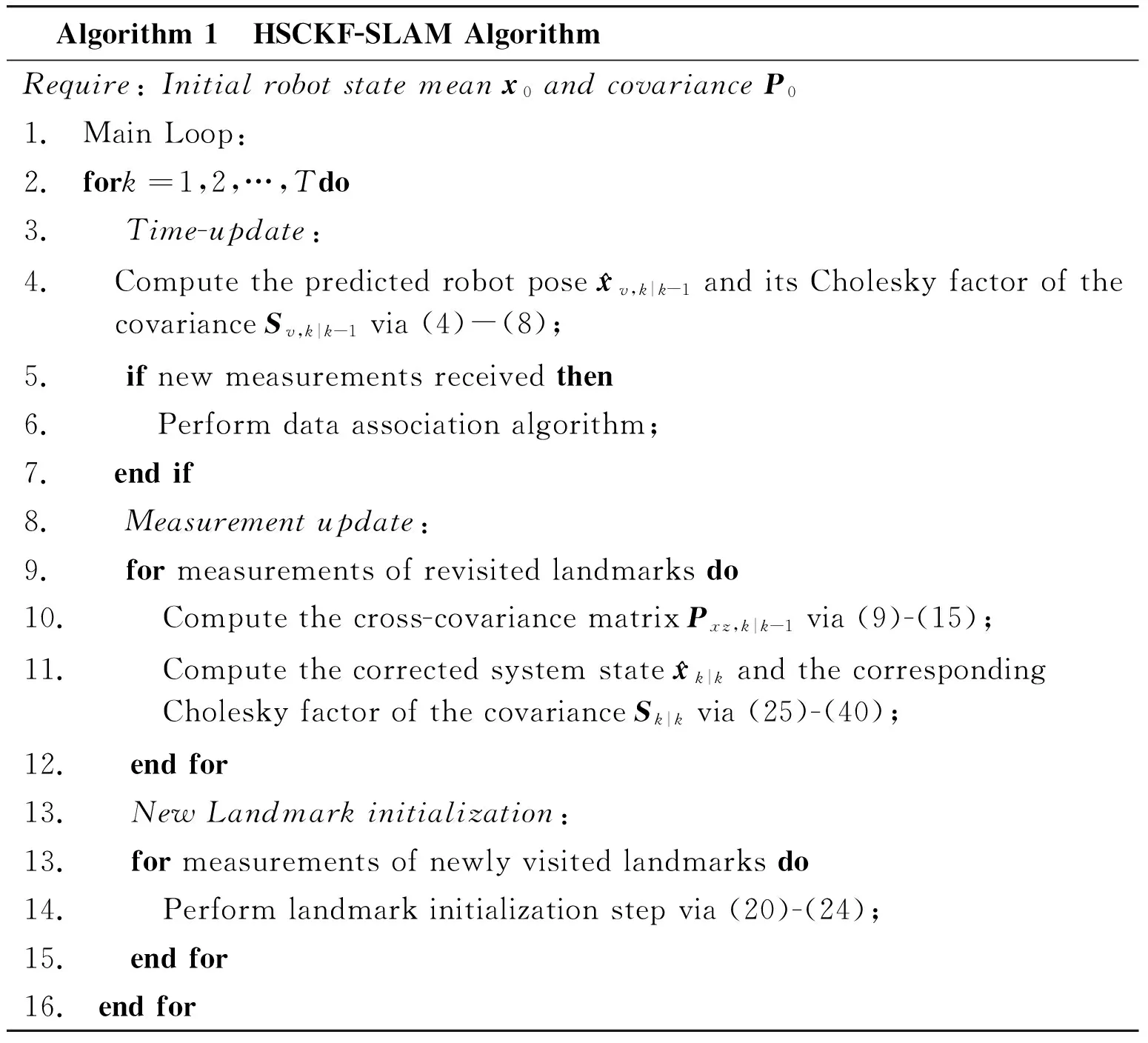
Algorithm1 HSCKF-SLAMAlgorithmRequire:Initialrobotstatemeanx0andcovarianceP01. MainLoop:2. fork=1,2,…,Tdo3. Time-update:4. Computethepredictedrobotpose^xv,k|k-1anditsCholeskyfactorofthecovarianceSv,k|k-1via(4)-(8);5. ifnewmeasurementsreceivedthen6. Performdataassociationalgorithm;7. endif8. Measurementupdate:9. formeasurementsofrevisitedlandmarksdo10. Computethecross-covariancematrixPxz,k|k-1via(9)-(15);11. Computethecorrectedsystemstate^xk|kandthecorresponding CholeskyfactorofthecovarianceSk|kvia(25)-(40);12. endfor13. NewLandmarkinitialization:13. formeasurementsofnewlyvisitedlandmarksdo14. Performlandmarkinitializationstepvia(20)-(24);15. endfor16. endfor

4 Simulations and results

A series of simulations have been conducted to evaluate the performance of the proposed HSCKF-SLAM algorithm in comparison with the UKF-SLAM and the SCKF-SLAM. The publicly available UKF-SLAM simulator*https://svn.openslam.org/data/svn/bailey-slam/is modified as a benchmark platform.The other two algorithms have been implemented in Matlab R2012a on a 2.9GHz Intel Corei7-3520M Processor. As presented in Fig.1(a), the robot is assumed to move along the predefined trajectory in a rectangular plane. The robot starts from the origin of the

global frame and detectsnearby landmarks with a laser sensor.The additive measurement noise is assumed to follow a Gaussian mixture distribution of the form:

0≤α≤1, σ2=βσ1

where α represents the noise model contamination, σ1and σ2are the standard deviations of the Gaussian mixture components, and β denotes the ratio between them.The process noise is 0.2m/s in wheel velocity and 2° in steering angle.Other simulation parameters are listed in Table 1.

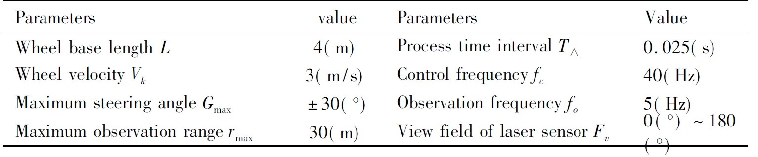
Table 1 Simulation parameters.

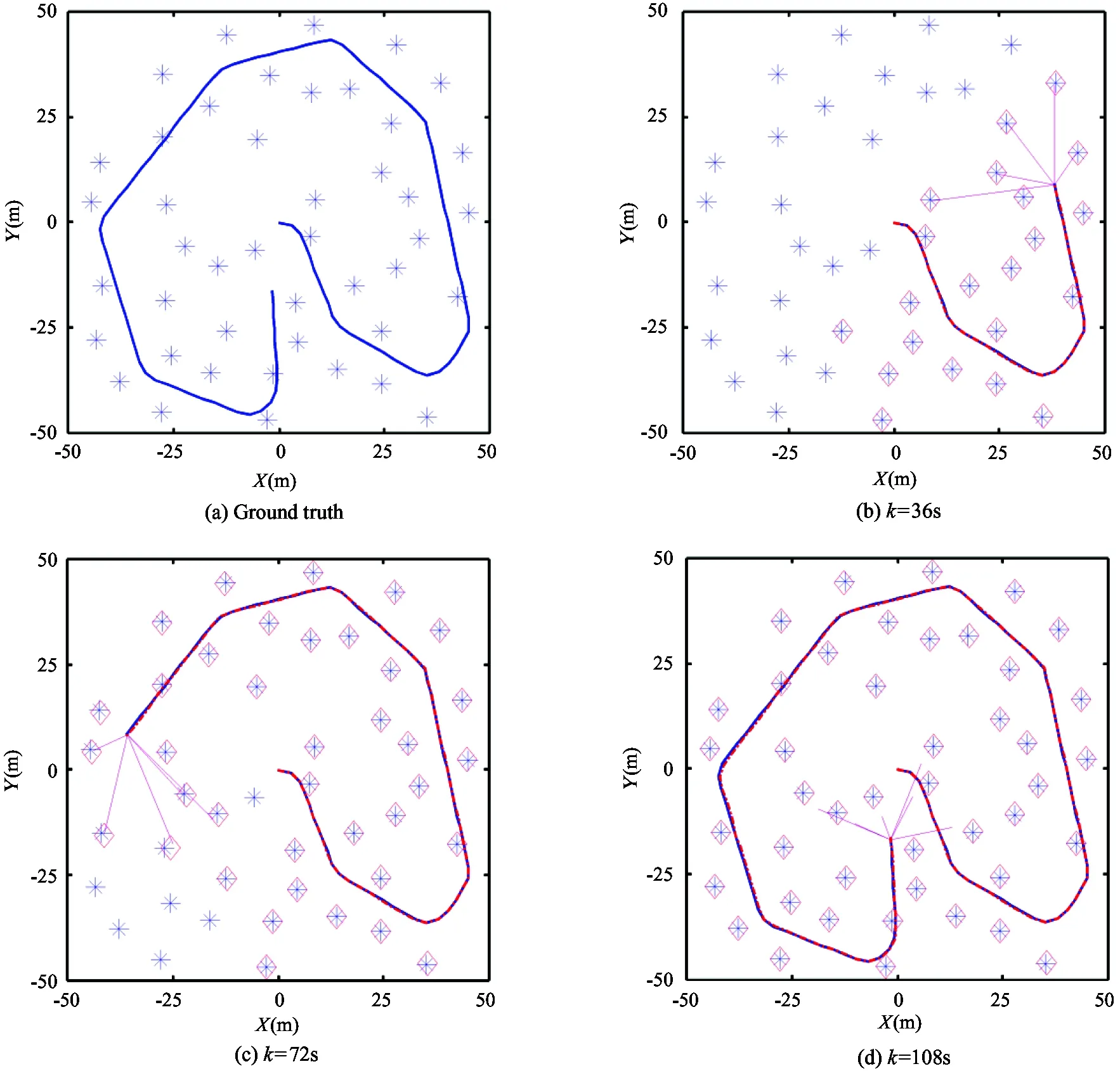
Fig.1 The simulation results.True landmark (*) and robot path (thick solid lines), estimated landmark (diamonds)

In order to evaluate the performance of the proposed algorithm under various measurement noise conditions,two simulation scenarios with different measurement noise models are considered: a Gaussian mixture contaminated noise model and an outlier contaminated noise model.For a fair comparison, all the SLAM algorithms are carried out with the same simulation parameters except that of the measurement noise.200 independent Monte Carlo simulation runs are conducted for each simulation scenario.

4.1 Results in Gaussian mixture contaminated noise case

In this simulation scenario,the measurement noise is assumed as a contaminated Gaussian model with two independent Gaussian mixtures. The standard deviation

of the main mixture component σ1is set to 0.2m in range and 2° in bearing. Fig.1(b)～(d) show the results of a typical simulation run where the contamination and ratio parameters are set to 0.3 and 10, respectively. These plots indicate that both the robot trajectories and landmarks are estimated accurately at different time steps (k=36s, 72s, and 108s) by the proposed algorithm. The Kalman gain weights under different measurement residuals are also presented in Fig.2. It can be seen that the weights reach local minimums in the most time steps when either the range measurement residual or the bearing measurement residual is a high peak of the curve. Moreover， larger measurement residuals can bring about smaller weights. As a result, the measurement outliers are supressed to a great extent in the Kalman update process.

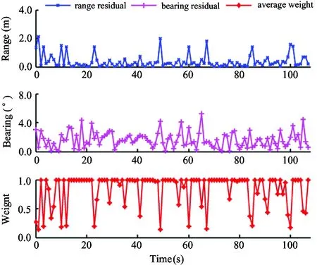
Fig.2 Average Kalman gain weights under different measurement residuals

The effects of different combinations of parameters α and β on accuracy are illustrated in Fig.3 and Fig.4. Fig.3 shows the relations between the average RMSE of the algorithms and contamination parameter α when ratio parameter β is fixed to 5. Similarly, the relations between average RMSE and ratio parameter β are shown in Fig.4, where α is set to 0.4. As observed in the figures, the HSCKF-SLAM outperforms the other algorithms in all cases. Besides, the superiority of the HSCKF-SLAM is more obvious as the parameters increase.The results indicate that the Huber based update plays a more important role when the distribution of the non-Gaussian noise has thicker tails. The SCKF-SLAM exhibits slightly better performance than the UKF-SLAM due to the reason that SCKF can approximate the nonlinear functions in higher order than UKF.The unscented transformation is no longer numerically stable and the Cholesky decomposition of the state covariance encounters troubles in cases of extremely large noise.

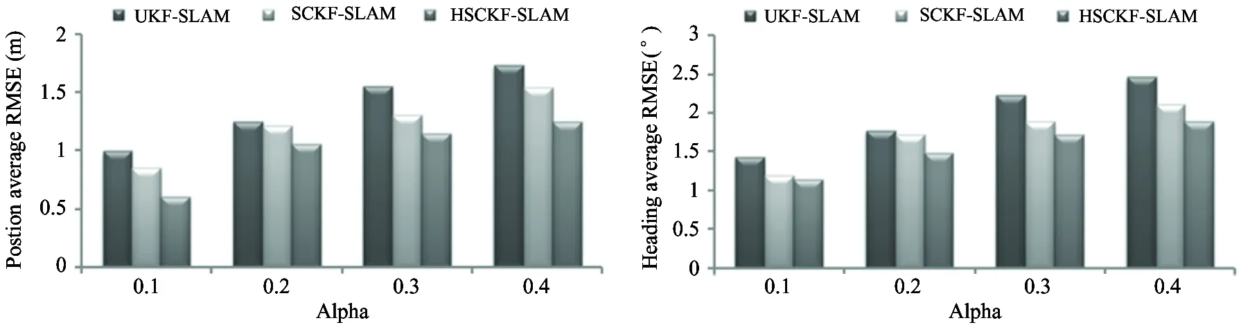
Fig.3 Average RMSE under different contamination parameters

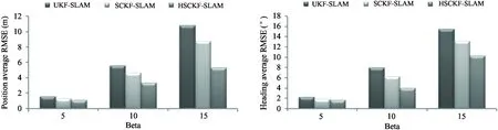
Fig.4 Average RMSE under different ratio parameters

4.2 Results in outlier contaminated noise case

In this simulation scenario, the basic measurement noise follows a Gaussian distribution by setting contamination parameter to 0. This Gaussian noise model is then contaminated by a number of random measurement outliers which are induced periodically. Totally 21 measurements are selected and biased by an offset [5m, 5°]. Fig.5 depicts RMSE of the robot position and heading of the algorithms. It can be seen from the results that both the UKF-SLAM and the SCKF-SLAM suffer from estimation errors larger than the HSCKF-SLAM apparently. The position and heading RMSE are below 1m and 1.2° for HSCKF-SLAM.This proves that HSCKF-SLAM can detect all the measurement outliers and reduce their influence effectively. The average NEES of the outlier scenario are shown in Fig.6, where the two horizontal dashed lines are plotted to mark the 95% two-side confidence region.It can be seen that both SCKF-SLAM and UKF-SLAM become inconsistent for all the time steps, while HSCKF-SLAM retains consistent for more than 75 time steps.These results demonstrate that by making use of Huber’s update method, the conventional Kalman type filter is insensitive to the measurement outliers.

Fig.5 Comparison of RMSE in outlier contaminated Gaussian measurement noise case

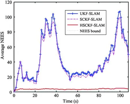
Fig.6 Average NEES of the robot position in outlier case

4.3 Computational cost

The computational costs of these algorithms are also compared. As illustrated in Table 2, UKF-SLAM requires the minimum computational cost. SCKF-SLAM demands more running time because QR decompositions are employed to ensure numerical stability. HSCKF-SLAM takes the most computational effort due to the extra realization of robust linear regression in the measurement update stage. However, the increased average running time for one single update step with Huber’s method is of the order of a 3ms.This increase is a worthwhile price to be paid for robustness and consistency. Besides, such a level of increase is often acceptable in real-time SLAM applications.

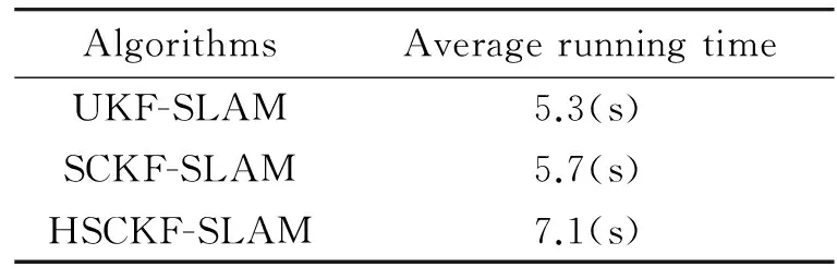
Table 2 Computational cost of algorithms

5 Conclusions

A robust SLAM algorithm based on SCKF and Huber’s GM-estimator is proposed for robot systems with non-Gaussian measurement noises. The integration of a GM-estimator doesn’t only retain the accurate merit of SCKF, but also provides an efficient way to work in non-Gaussian cases, with performance surpassing the benchmark algorithms in robustness and consistency.The influence of Huber’s GM-estimator on the convergence rate and efficiency properties with different score functions will be further studied and optimized.

Reference

[ 1] Dissanayake M W M G, Newman P, Clark S, et al. A solution to the simultaneous localization and map building (SLAM) problem.IEEETransactionsonRoboticsandAutomation, 2001, 17(3): 229-241

[ 2] Durrant-Whyte H, Bailey T. Simultaneous localization and mapping: Part I.IEEERoboticsandAutomationMagazine, 2006, 13(2): 99-108

[ 3] Martinez-Cantin R, Castellanos J A. Unscented SLAM for large-scale outdoor environments. In: Proceedings of the International Conference on Intelligent Robots and Systems, Edmonton, Canada, 2005. 328-333

[ 4] Chandra K P B, Gu D, Postlethwaite I. A cubature H∞ filter and its square-root version.InternationalJournalofControl, 2014, 87(4): 764-776

[ 5] Arasaratnam I, Haykin S. Cubature Kalman filters.IEEETransactionsonAutomaticControl, 2009, 54(6): 1254-1269

[ 6] Gandhi M A, Mili L. Robust Kalman filter based on a generalized maximum-likelihood-type estimator.IEEETransactionsonSignalProcessing, 2010, 58(5): 2509-2520

[ 7] Li X R, Jilkov V P. Survey of maneuvering target tracking. Part V. Multiple-model methods.IEEETransactionsonAerospaceandElectronicSystems, 2005, 41(4): 1255-1321

[ 8] Zoubir A M, Koivunen V, Chakhchoukh Y, et al. Robust estimation in signal processing: A tutorial-style treatment of fundamental concepts.IEEESignalProcessingMagazine, 2012, 29(4): 61-80

[ 9] Montemerlo M, Thrun S, Koller D, et al. FastSLAM: A factored solution to the simultaneous localization and mapping problem. In: Proceedings of the National Conference on Artificial Intelligence, Edmonton, Canada, 2002. 593-598

[10] Ahmad H, Namerikawa T. Feasibility study of partial observability in H∞filtering for robot localization and mapping problem. In: Proceedings of the 2010 American Control Conference, Baltimore, USA, 2010.3980-3985

[11] Huber P J. Robust Statistics. New Jersey: John Wiley & Sons, 2004. 43-48

[12] Karlgaard C D, Schaub H. Huber-based divided difference filtering.JournalofGuidance,Control,andDynamics, 2007, 30(3): 885-891

[13] Chang L, Hu B, Chang G, et al. Huber-based novel robust unscented Kalman filter.IETScience,Measurement&Technology, 2012, 6(6): 502-509

[14] Wang X, Cui N, Guo J. Huber-based unscented filtering and its application to vision-based relative navigation.IETRadar,SonarandNavigation, 2010, 4(1): 134-141

[15] Coleman D, Holland P, Kaden N, et al. System of subroutines for iteratively reweighted least squares computations.ACMTransactionsonMathematicalSoftware, 1980, 6(3): 327-336

[16] Hampel F R, Ronchetti E M, Rousseeuw P J, et al. Robust Statistics: the Approach Based on Influence Functions. Published Online, John Wiley & Sons, 2011. 307-341

Xu Weijun， born in 1985. He is a Ph.D. candidate in the College of Biomedical Engineering and Instrument Science of Zhejiang University. His main research fields arerobot simultaneous localization and mapping, multiple target tracking and multi-agent navigation.

10.3772/j.issn.1006-6748.2016.01.006

① Supported by the National High Technology Research and Development Program of China (2010AA09Z104), and the Fundamental Research Funds of the Zhejiang University (2014FZA5020).

② To whom correspondence should be addressed. E-mail: rongxinj@zju.edu.cnReceived on Dec. 3， 2014