
Bending modes and transition criteria for a flexible fiber in viscous flows*
2016-12-26 06:51XiufengYANG杨秀峰MoubinLIU刘谋斌
水动力学研究与进展 B辑 2016年6期
Xiufeng YANG (杨秀峰), Mou-bin LIU (刘谋斌)
1. Institute of Mechanics, Chinese Academy of Sciences, Beijing 100190, China
2. Department of Mechanical Engineering, Iowa State University, Ames, IA 50011, USA, E-mail: xyang@iastate.edu
3. BIC-EAST, College of Engineering, Peking University, Beijing 100871, China
4. State Key Laboratory for Turbulence and Complex systems, Peking University, Beijing 100871, China
Bending modes and transition criteria for a flexible fiber in viscous flows*
Xiufeng YANG (杨秀峰)1,2, Mou-bin LIU (刘谋斌)3,4
1. Institute of Mechanics, Chinese Academy of Sciences, Beijing 100190, China
2. Department of Mechanical Engineering, Iowa State University, Ames, IA 50011, USA, E-mail: xyang@iastate.edu
3. BIC-EAST, College of Engineering, Peking University, Beijing 100871, China
4. State Key Laboratory for Turbulence and Complex systems, Peking University, Beijing 100871, China
The present paper follows our previous work in which a coupling approach of smoothed particle hydrodynamics (SPH) and element bending group (EBG) was developed for modeling the interaction of viscous incompressible flows with flexible fibers. It was also shown that a flexible object may experience drag reduction because of its reconfiguration due to fluid force on it. However, the reconfiguration of deformable bodies does not always result in drag reduction as different deformation patterns can result in different drag scales. In the present work, we studied the bending modes of a flexible fiber in viscous flows using the presented SPH and EBG coupling approach. The flexible fiber is immersed in a fluid and is tethered at its center point, while the two ends of the fiber are free to move. We showed that the fiber undergoes four different bending modes: stable U-shape, slight swing, violent flapping, and stable closure modes. We found there is a transition criterion for the flexible fiber from slight swing, suddenly to violent flapping. We defined a bending number to characterize the bending dynamics of the interaction of flexible fiber with viscous fluid and revealed that this bending number is relevant to the non-dimensional fiber length. We also identified the critical bending number from slight swing mode to violent flapping mode.
smoothed particle hydrodynamics (SPH), fluid-structure interaction, flexible fiber, drag reduction
Introduction
Fluid-structure interaction is one of the key topics in fluid mechanics. The dynamics of a flexible object in a fluid is fundamentally important in engineering and sciences[1-3]. An object moving through a viscous fluid experiences a drag force due to its interaction with the fluid. Newton originally studied the drag force acting on an object with the fluid flows around it[4]. For a rigid object, the drag force is proportional to the square of the relative velocity of the object tothe fluid at large Reynolds numbers. However, for a flexible object that can bend in the flow direction, the drag may increase slower than the square of the velocity because of the reconfiguration of the object caused by fluid forces[5-7]. Drag reduction with flexible objects can be frequently observed in plant growth[5,8], animal movement[2,9], and even in vehicle design[10]. The reduction in drag on a flexible body is due to the reconfiguration of the body, as the reconfiguration makes the frontal area facing the flow become smaller and makes the shape of the body more streamlined with smaller drag coefficient. Therefore, how a flexible fiber changes its shape while moving in viscous fluids is critical for drag reduction.
According to Yang et al.[11], the bending modes of the center point-tethered flexible fiber in a viscous flow can be identified as: the U-shaped mode, the flapping mode, and the closed mode. Many literature have been focused on the U-shaped mode and the corresponding drag scaling law, including experiments[6,7]and numerical modeling[12]. However, the dragscaling law for different bending modes may be different[11], but few of literature was focused on the bending modes of flexible fibers in viscous fluids and the transition between the bending modes.
In our previous work[11], the classification of the bending modes of a flexible fiber in a fluid is a little bit oversimplified as the free end of the flexible fiber can lead to more detailed patterns. Therefore, in the present work, we focus on the deformation patterns of the flexible fiber as the drag reduction is closely related to the deformation patterns of the fiber. The present paper will extend the bending modes and find the corresponding transition criteria.
A coupled method[11,13,14]of smoothed particle hydrodynamics (SPH)[15,16]and element bending group (EBG)[17]is used to model the interaction of viscous fluids with flexible fiber. SPH particles are used to model the viscous fluid flow governed by Navier-Stokes equations, and EBG particles are used to model the dynamic movement and deformation of flexible fibers. The interaction of the neighboring fluid (SPH) and fiber (EBG) particles renders the interaction of fluid and flexible fiber[11,14]. In numerical simulation, the flexible fiber is immersed in a fluid and is tethered at its center point, while the two ends of the fiber are free to move.
1. Numerical method
The interaction of flexible fiber and viscous flow is very complex. In order to model the process of flexible fiber interacting with fluid flow, the SPH method is applied to simulate fluid flow, while the EBG method is applied to simulate the flexible fiber.

Fig.1 Sketch of the computational settings. The midpoint of the fiber is fixed in the midline of the channel, while the two ends of the fiber are free to move
1.1 Problem set-up
The computational setting for the modeling of fiber-fluid interaction is shown in Fig.1. A one-dimensional flexible fiber is immersed in a two-dimensional viscous fluid channel. The midpoint of the fiber is fixed in the midline of the channel, while the two ends of the fiber are free to move. The system is initially at rest, and then the fluid is driven by a body forceg . The upper and lower boundaries are solid walls. The left and right boundaries are flow inlet and outlet. They are treated as periodic boundary condition. A layer of porous media is deployed in the inlet area to remove wave energy and vortices from the exit area and makes the inlet velocity uniform.
1.2 Methodology
A brief introduction of the numerical method used in this paper is given in this section. For more details about the SPH-EBG method, please refer to [11,13,14].
In SPH method, fluid is replaced by a set of particles, which possess individual material properties. The SPH particles move according to fluid governing conservation equations and they also act as the computational frame for field variable approximations. The SPH equations for viscous fluid can be written in the following form


where sabis the strength of the force acting between particlesaandb .
In order to calculate pressure, the following equation ofstate[18,19]is used

where ρ0is a reference density,cis a numerical speed of sound.
The flexible fiber is modeled by using the EBG method. An EBG is made of two adjacent line segments connecting three neighboring particles. The bending moments on the segments are transformed to pairs of forces acting on particles[11,13,14,17].
According to Newton’s second law of motion, the equation for a flexible fiber particle can be written as follows

whereT denotes the tension acting on a fiber particle from adjacent fiber particles,FBdenotes the bending force due to EBG bending moment,FDdenotes the fluid force.
The tension is defined as

whereEandA are the Young’s modulus and the cross-sectional area of the fiber, respectively.is the reference distance between fiber particlesaandb.
The bending force is defined as

where Madenotes the moment acting on particlea.
In implementing the fluid-fiber interaction, the SPH particles and EBG particles are treated as neighboring particles which contribute in the SPH approximation. The contribution of EBG (fiber) particles to the approximation of SPH (fluid) particles leads to the force on fluid particles from fiber and the contribution of fluid particles to the approximation of fiber particles produces force on fiber particles from fluid. Therefore EBG particles can be regarded as a special type of SPH particles. On one hand, EBG particles interact with neighboring EBG particles with tension and bending forces. On the other hand, they have SPH approximation with contribution from neighboring fluid (ordinary) particles and also contribute in SPH approximation of neighboring fluid particles.
2. Bending modes
The shape of the flexible fiber changes during its interaction with surrounding fluid and the reconfiguration of the fiber is closely related to the flow velocity. Figure 2 shows four typical bending modes of a flexible fiber with gradual increase in the flow velocity: (a) the U-shaped mode, (b) the swing mode, (c) the flapping mode, and (d) the closed mode. In the case shown in Fig.2, the length(L)and bending rigidity (EI)of the fiber are 0.05 m and 0.001 Jm, respectively. The density(ρ)and kinetic viscosity(µ) of the fluid are 1 000 kg/m3and 0.004 Ns/m2, respectively.

Fig.2 Four typical bending modes of a flexible fiber and the flow structures behind the fiber at different flow velocities. The color shows the angular velocity of SPH particles
It is shown in Fig.2 that when the flow initiates, the fiber begins to bend and forms a streamlined U shape-like the letter “U” (Fig.2(a)). The U-shaped mode maintains when the flow velocity is less than about 1 m/s. When the flow velocity increases to around 1 m/s-2.5 m/s, the fiber bends more, also basically in a U-shape, but its two free ends begin to oscillate slightly due to vortex shedding (Fig.2(b)). With further increase in the flow velocity to 2.5 m/s-4 m/s, the fiber suddenly flaps violently with large amplitude (Fig.2(c)). The flapping of the fiber is also caused by vortex shedding with much stronger influence. This is similar to a flag flapping in wind. At last, both free ends of the fiber overlap and form a closed shape, like a tadpole (Fig.2(d)).
Figure 3 shows the y-coordinates of the two free ends of the fiber (y1and y2), the profile lengthsin the flow direction (Lx)and the direction perpendicular to the flow(Ly), as functions of flow velocity. The length and bending rigidity of the fiber are 0.05 m and0.001 Jm,respectively.The density and kinematic v iscosity of the fluid are 1 000 kg/m3and 0.004 Ns/m2respectively. It is shown in Fig.3 that transitions occur from slight swing to violent flapping at flow velocity around 2.5 m/s and from violent flapping to closure at flow velocity around 4 m/s.

Fig.3 The y -coordinates (y1and y2) of the free ends and the profile lengths of the fiber inx direction (Lx)and y direction (Ly)varying with flow velocity. The inset shows the transition from slight swing to large flapping
Both the swing mode and the flapping mode are caused by vortex shedding. However, the amplitude of the flapping mode is much larger than that of the swing mode, as shown in Fig.3. Another difference between these two modes is that at the swing mode as shown in Fig.2(b), the whole fiber swings around the fixed point of the fiber as a simple pendulum, while at the flapping mode as shown in Fig.2(c), the two free ends of the fiber flap around different points, somewhere between the fixed point and the free end of the fiber.
In the flapping mode, the fiber moves violently. A very likely reason is that resonance occurs, that is, the frequency of the vortex shedding is very close to the flapping frequency of the fiber. The fluid drag force on the fiber also increases quickly as the flapping amplitude of the fiber increases. Therefore, the amplitude does not continue to increase when it reaches a certain level.
3. Transition criteria
It is clearly shown in Fig.3 that there are two transition points between the bending modes. The first point is the transition from the swing mode to the flapping mode (around the velocity of 2.5 m/s) and the second is the transition from the flapping mode to the closed mode (around the velocity of 4 m/s).
It is reasonable that the bending mode of the flexible fiber is up to its ability to bend and the fluid force acting on it. Hence a non-dimensional number is defined as
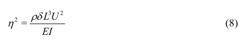
whereρandU are the density and average velocity of the viscous flow, respectively,δ,LandEI are the thickness, length and bending rigidity of the fiber, respectively.ηwas referred to as the nondimensional flow speed[6]. However, as the fluid drag acting on a fiber is proportional to ρδLU2and the bending force of the fiber is proportional toEI/ L2, η2is actually the ratio of the drag force to the bending force. Thereforeηis herein defined as Bending number, which can be used to characterize the bending dynamics of a flexible fiber interacting with viscous fluids. Like the Reynolds number in characterizing viscous flows, this bending number can be used to judge the similarity of systems with interacting viscous fluid and fibers. In another words, for two systems of interacting viscous fluid and fibers, if the bending number is the same, the corresponding flow patterns should be the same.
It is also straightforward to define another parameter, non-dimensional length, as

which is the ratio of the profile length in flow direction (Lx)to the whole length of the fiber(L). It also reflects the bending degree of the flexible fiber. If assuming the fiber to be incompressible and inextensible,
λis expected to be equal to 0 when the fiber do not bend at all and approaches 0.5 when the fiber is totally folded about its center point.
By using these two non-dimensional numbers, it is feasible to further investigate the bending dynamics and the mode transition for a system with interacting viscous fluid and fibers at different scenarios. Figure 4 shows the critical parametersλ∗andη∗at which the flexible fiber flaps with large amplitudes as a function of fiber length, bending rigidity, and fluid density. The fluid densities of Cases (a)-(d) are all 1 000 kg/m3. The fiber bending rigidities of Cases (a), (b), (e) and (f) are all 0.001 Jm. The fiber lengths of Cases (c)-(f) are all 0.04 m. It is shown in Fig.4 that when the violent flapping state of flexible fibers appears,λandηare about 0.44 and 28, respectively.Therefore the transition criterion for the flexible fiber from the swing mode to the flapping mode isλ∗≈0.44 or η∗≈28.

Fig.4 The critical bending numbers(η∗)and non-dimensional profile fiber lengths(λ∗)for the transition from slight oscillation to large flapping versus fiber lengths(L), fiber bending rigidities(EI)and fluid densities(ρ)
As bothλandηcan characterize the bending degree or bending dynamics of a fiber in a fluid-fiber flow system, it is possible that there exists some kind of link between them. A simple analysis shows that λincreases asηincreases: the increase ofηmeans that the fluid drag force on the fiber increases when the bending force of the fiber keeps unchanged, thus the fiber bends more whenηincreases, whileλincreases as the fiber bends more. Further studies reveal thatλandηare inherently related. By fitting the data from numerical simulation, we can obtain the following empirical formula for a flexible fiber in the U-shape state

wherea andβare parameters, and C≤ max(λ)= 0.5. If the fiber is folded in half,λis equal to 0.5. However, because the bending rigidity of the fiber is larger than zero, the flow cannot fold it totally in half. There is always a circle near the fixed center of the fiber, as shown in Fig.2(d). Therefore,λis less than 0.5 and Cis also less than 0.5. For most of the cases in our simulations, the value ofC is about 0.46.
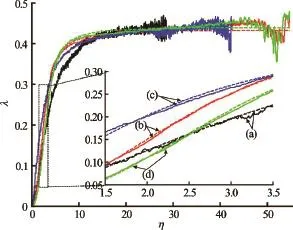
Fig.5 Comparison of fitted function and numerical data: nondimensional profile fiber length(λ)versus non-dimensional flow velocity(η). The solid lines are numerical data, and the dash lines are fitted curves
The comparison of fitted function and numerical data of four different cases are shown in Fig.5. For the case in Fig.5(a), the fiber length is 0.03 m, the fiber bending rigidity is 0.001 Jm, and the fluid density is 1 000 kg/m3. For the case in Fig.5(b), the fiber length is 0.04 m, the fiber bending rigidity is 0.0001 Jm, and the fluid density is 1 000 kg/m3. For the case in Fig.5(c), the fiber length is 0.05 m, the fiber bending rigidity is 0.001 Jm, and the fluid density is1 000 kg/m3. For the case in Fig.5(d), the fiber length is 0.06 m, the fiber bending rig3idity is 0.001 Jm, and the fluid density is 3 000 kg/m. Figure 5 shows that Eq.(10) agrees with numerical data very well. If the value ofλapproachesC, the fiber will flap violently and later form a closed shape.
4. Conclusion
In this work, the bending dynamics of flexible fibers are investigated numerically by using a particlebased model, in which SPH and EBG is coupled for modeling the interaction of viscous fluids with flexible fibers. During the fiber-fluid interaction process, the fiber exhibits four different bending modes, namely, the stable U-shape mode, the slight swing mode, the violent flapping mode, and the final closed mode. The bending dynamics of a flexible fiber can be characterized using a bending number, which reflects the ratio of the drag force to the bending force. The transition criterion for the flexible fiber from the swing mode to the flapping mode is λ≈0.44or η≈28. It revealed that the bending number is inherently related to the non-dimensional fiber length, through an empirical formula.
[1] Shelley M. J., Zhang J. Flapping and bending bodies interacting with fluid flows [J]. Annual Review of Fluid Mechanics, 2011, 43(1): 449-465.
[2] Liao J. C., Beal D. N., Lauder G. V. et al. Fish exploiting vortices decrease muscle activity [J]. Science, 2003, 302(5650): 1566-1569.
[3] Jung S., Mareck K., Shelley M. et al. Dynamics of a deformable body in a fast flowing soap film [J]. Physical Review Letters, 2006, 97(13): 134502.
[4] Von Karman T. Aerodynamics: Selected topics in the light of their historical development [M]. New York, USA: Courier Dover Publications, 2004.
[5] Vogel S. Drag and reconfiguration of broad leaves in high winds [J]. Journal of Experimental Botany, 1989, 40(8): 941-948.
[6] Alben S., Shelley M., Zhang J. Drag reduction through self-similar bending of a flexible body [J]. Nature, 2002, 420(6915): 479-481.
[7] Gossellin F., De Langre E., Machado-Almeida B. A. Drag reduction of flexible plates by reconfiguration [J]. Journal of Fluid Mechanics, 2010, 650(1): 319-341.
[8] Albayrak I., NIKORA V., Miler O. et al. Flow-plant interactions at leaf, stem and shoot scales: drag, turbulence, and biomechanics [J]. Aquatic Sciences, 2014, 76(2): 269-294.
[9] Ristroph L., Zhang J. Anomalous hydrodynamic drafting of interacting flapping flags [J]. Physical Review Letters, 2008, 101(19): 194502.
[10] Stanford B., Ifju P., Albertani R. et al. Fixed membrane wings for micro air vehicles: Experimental characterization, numerical modeling, and tailoring [J]. Progress in Aerospace Sciences, 2008, 44(4): 258-294.
[11] Yang X., Liu M., Peng S. Smoothed particle hydrodynamics and element bending group modeling of flexible fibers interacting with viscous fluids [J]. Physical Review E, 2014, 90(6): 063011.
[12] Alben S., Shelley M., Zhang J. How flexibility induces streamlining in a two-dimensional flow [J]. Physics of Fluids, 2004, 16(5): 1694-1713.
[13] Hosseini S. M., Feng J. J. A particle-based model for the transport of erythrocytes in capillaries [J]. Chemical Engineering Science, 2009, 64(22): 4488-4497.
[14] Yang X., Liu M., Peng S. et al. Numerical modeling of dam-break flow impacting on flexible structures using an improved SPH-EBG method [J]. Coastal Engineering, 2016, 108(1): 56-64.
[15] Gingold R. A., Monaghan J. J. Smoothed particle hydrodynamics: Theory and application to non-spherical stars [J]. Monthly Notices of the Royal Astronomical Society, 1977, 181(3): 375-389.
[16] Liu M. B., Liu G. R. Smoothed particle hydrodynamics (SPH): An overview and recent developments [J]. Archives of Computational Methods in Engineering, 2010, 17(1): 25-76.
[17] Zhou D., Wagoner R. Development and application of sheet-forming simulation [J]. Journal of Materials Processing Technology, 1995, 50(1-4): 1-16.
[18] Morris J. P., Fox P. J., Zhu Y. Modeling low Reynolds number incompressible flows using SPH [J]. Journal of Computational Physics, 1997, 136(1): 214-226.
[19] Liu M. B., LI S. M. On the modeling of viscous incompressible flows with smoothed particle hydrodynamics [J]. Journal of Hydrodynamics, 2016, 28(5): 731-745.
(Received June 20, 2016, Revised September 28, 2016)
* Project supported by the National Natural Science Foundation of China (Grant Nos. 11302237, 11172306 and U1530110).
Biography:Xiufeng YANG (1985-), Male, Ph. D.,
Assistant Professor
Mou-bin LIU,
E-mail: mbliu@pku.edu.cn

- 水动力学研究与进展 B辑的其它文章
- Energy saving by using asymmetric aftbodies for merchant ships-design methodology, numerical simulation and validation*
- Development of Cartesian grid method for simulation of violent ship-wave interactions*
- Numerical study on the effects of progressive gravity waves on turbulence*
- Experimental tomographic methods for analysing flow dynamics of gas-oilwater flows in horizontal pipeline*
- Coupling of the flow field and the purification efficiency in root system region of ecological floating bed under different hydrodynamic conditions*
- Modelling hydrodynamic processes in tidal stream energy extraction*