Recover Implied Volatility in Short-term Interest Rate Model

XU Zuo-liang

(1.School of Mathematics and Statistics,Shandong Normal University,Jinan 250014,China;2.School of Information,Renmin University of China,Beijing 100872,China)

§1.Introduction

Derivative security for interest rate is one whose payoffis determined by interest rate to some extent[1].Recently,in financial market,the pricing of interest rate derivatives become a very important research work.One of the most widely used classes of valuation models is the short-term interest rate model,such as CIR model[2]and Hull-While model[3].The short-term interest model is an indispensable tool for the derivatives pricing and risk management.In order to pricing more accurately,calibration of the model parameters to specific market data is required.Much research has been done on the analysis of calibration of different parameters in different models[4-8].

As is known to us that volatilities of underlying assets have become widely used by corporate treasures as well as by risk controllers and financial institution in risk management,portfolio hedging and derivatives valuation.Since the volatilities of underlying assets cannot be directly observed in general,much research has been done on the inverse problem to reconstruct the implied volatility from market prices[9-11].In[9],Rainer gives the general structure of optimization in the context of calibration of stochastic models for interest rate derivatives.Based on the relevant market data,a novel numerical algorithm for the optimization of parameters in interest rate models is presented.In[10],Bouchouev et al.consider the problem of reconstruction of volatility from market prices of options with different strikes.As the volatility is only stock price dependent,a linearized version of the inverse problem is considered,a simple convenient representation of the linearization and a reliable numerical algorithm are obtained.

In this paper,we continue research of the linearization technique.By using linearization,we attempt to reconstruct the implied volatility of interest rate from the market prices of zerocoupon bond,which is sold in somewhat higher discount and will be redeemed on its face value on the maturity date.

Suppose that the behavior of short-term interest rateris modeled by the following stochastic differential equation

whereais a constant,W(t)denotes a standard Wiener process,θ(t)is a deterministic function of time,and the volatility factorσ(r)is a function of interest rate.

In practice,the spot rate is never less than zero and never greater than a certain number,which is assumed to beR.Therefore we assume that the interest rater∈Ω=[0,R].

We denote the value of zero-coupon bondv(t,r)is a function of current timetand interest rater.Following the general method for derivative security pricing[12],we get the partial differential equation for a zero-coupon bond in the form

whereω=[0,T]×[0,R],Tis the expiration date,a time-dependent functionλ(t)is market price for risk of interest rate which reflects the relationship between risk and yield,andσ(r)is the only parameter in the model that is unknown.

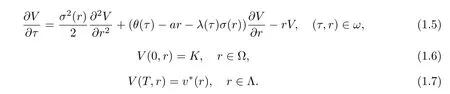
The final condition is given by

whereKis a certain face value of zero-coupon bond.

Now,one key problem for us is to reconstruct implied volatilityσ(r)from the observed market prices of zero-coupon bondv,which is described as the inverse problem of zero-coupon bond pricing.

Problem 1Given market prices of zero-coupon bond, find the implied volatility functionσ(r)such that the solution of(1.2)～(1.3)at initial timet=0 with different interest rates satis fies

wherev∗(r)denotes the current market price of zero-coupon bond at timet=0 andr∈Λ⊆Ω.

It is convenient to make the change of variableτ=T−tandV(τ,r)=v(t,r).For simplicity,we denoteθ(τ),λ(τ)still.Then equations(1.2)～(1.4)can be rewritten as follows

The remainder of the paper is organized as follows.In section 2,we simplify the partial differential equation by applying linearization approach and introduce the power series to derive the formulas of the price of zero-coupon bond.In section 3,an integral equation is formulated and in order to solve the problem,we address the regularization method.Numerical results are given in section 4.In section 5,some concluding remarks are given.

§2.Linearization

In this section, first we assume the volatility to be consisting of a given constant and a small perturbation,then based on the form of perturbation,we introduce the power series which play an important role for our reconstruction formulas.

2.1 Linearization at Constant Volatility

To recoverσ(r),we first assume

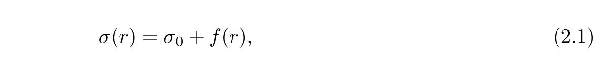
whereσ0is a given positive constant,the functionf(r)is a small perturbation ofσ0,and takes the form[13]

whereεis a sufficiently small positive constant andg(r)=0 outside Ω.

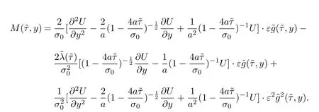
Substituting(2.1)and(2.2)into(1.5)gives

where

For simplification,by using the following substitution

where

and

Then we simplify equations(2.3),(1.6)and(1.7)to

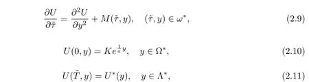
where

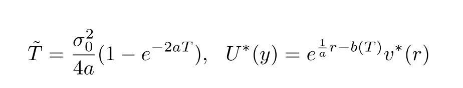
and

Hereω∗is the transformed intervalω.As(τ,r)∈ω,it is easy to find the intervalybelongs to denoted by Ω∗. Λ∗is the intervalybelongs to whenτ=Tandr∈Λ.

Problem 2GivenU∗(y), find the perturbation˜f(˜τ,y)such that the solution of(2.9)～(2.10)satis fies the condition(2.11)fory∈Λ∗.

2.2 Power Series

Recallingf(r)=εg(r)in(2.2),we considerUin power series of the parameterε[13].

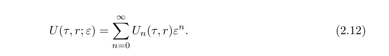
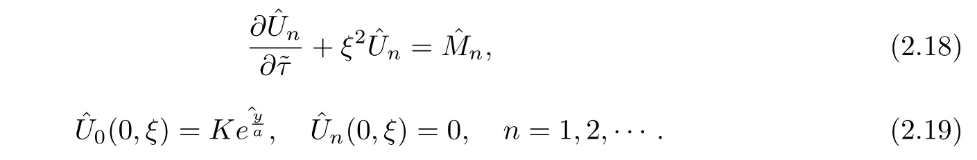
Substituting(2.12)into(2.9)and grouping terms in power ofε,we may derive recursion equations forUn

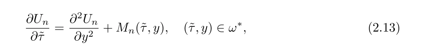
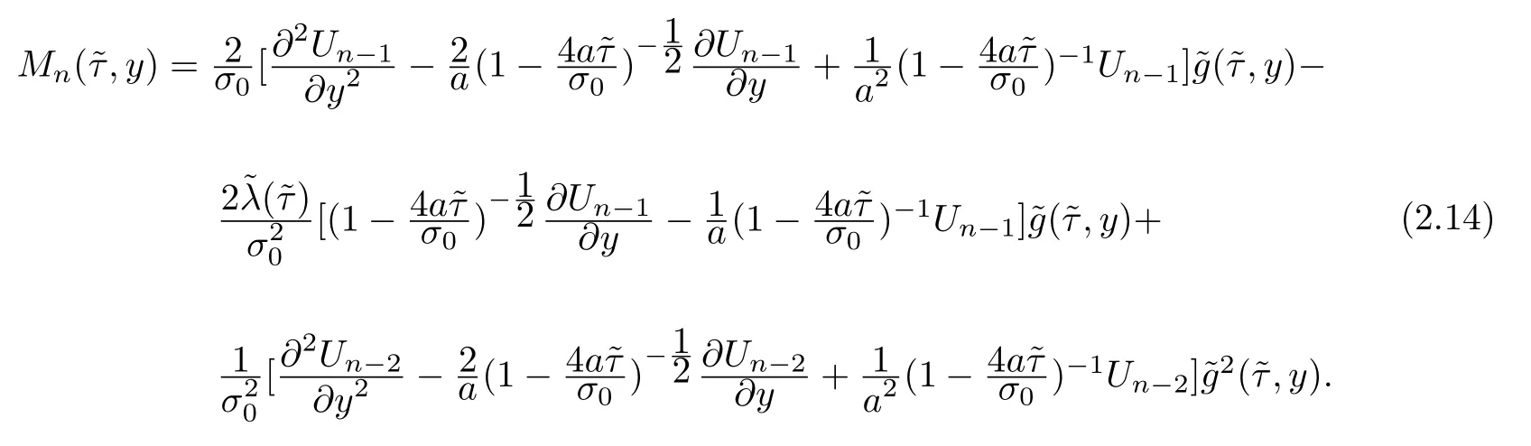
where

Inserting(2.12)into(2.10)gives the initial condition forUn

In the above recursion,it is understood thatUnis denoted as zero whenever the integern＜0.We notice that the transmission problem(2.13)～(2.15)for the current termsUninvolvesMn,which depend only on the previous two termsUn−1andUn−2.Thus,the problem(2.13)～(2.15)indeed can be solved efficiently in a recursive manner starting fromn=0.For each integern,it is easy to get the solution of the initial value problem of parabolic differential equations(2.13)～(2.15).

Lemma 1The solution of(2.13)～(2.15)is an integral equation as following

ProofGiven a functionu(x),the one-dimensional Fourier transform ofuis defined by

Taking the Fourier transform of(2.13)～(2.15)with respect toy,we have

Solving the initial value problem for the ordinary differential equation,we obtain

Taking the inverse Fourier transform of the above equation(2.20)with respect toξ,we can obtain the solution in the form of(2.16).

§3.The Linearized Inverse Problem and Regularization

In this section,neglecting high order terms in the power series,we formulate an integral equation about perturbationf(r).In order to solve the linearized inverse problem,we address Tikhonov regularization method[14].

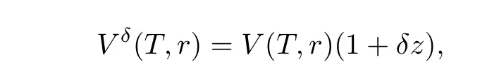
In the paper,we assume the observed market prices for zero-coupon bonds have some relative random noise.LetVδ(T,r)be the noisy data at timet=Tand it takes the form

whereV(T,r)denotes the noise-free data at timet=Tandδrepresents the noise level.

Under the change of variables(2.5),we have

It follows from the expression(2.12)that we have

Rearranging(3.3)yields

Neglecting the asymptotic terms ofε2andδin(3.4)gives

which plays an important role in the linearization of the inverse problem.

In the following,we will deduce the analytic expression of the order zero term and the order one term respectively from Lemma 1.

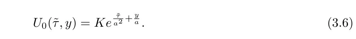
Order Zero TermRecalling(2.14),we have

Using the solution representation(2.16),we obtain

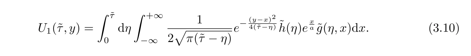
Order One TermInserting(3.7)into(2.14),we have

where

Using the solution representation(2.16),we have

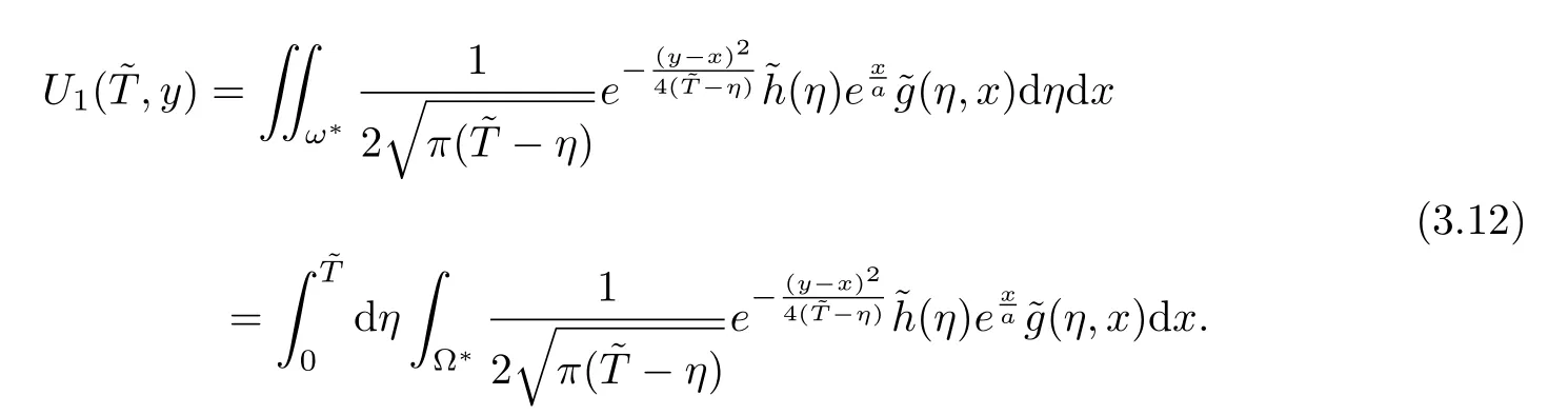
From variable substitution(2.5),Jacobian is obtained asJ=then we have

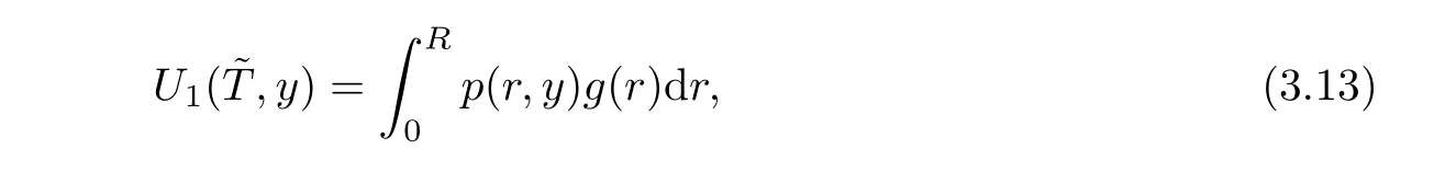
where

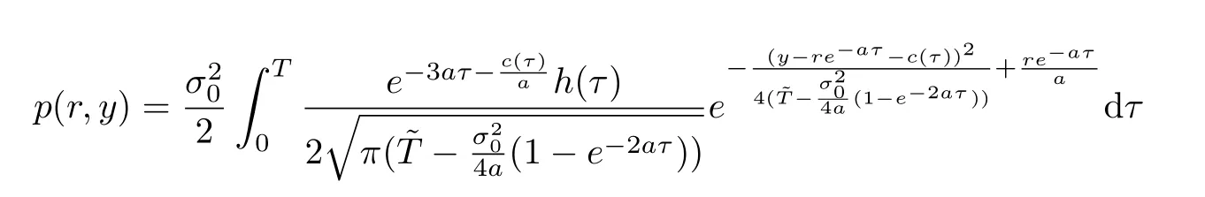
withh(τ)=

Inserting(3.13)into(3.5),we have an integral function as follows

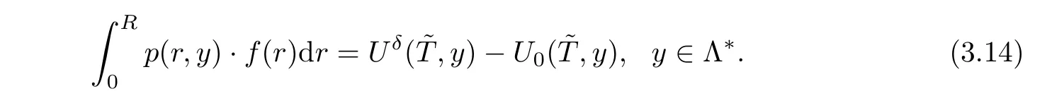
De fine an operatorAas follows

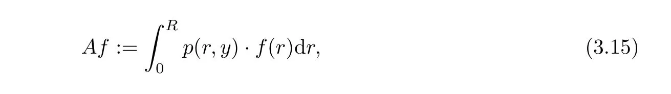
then we have

The equation(3.16)is a Fredholm integral equation of the first kind and is an ill-posed problem under noisy propagation.Here we use the Tikhonov regularization method which lies in minimization of the following functional

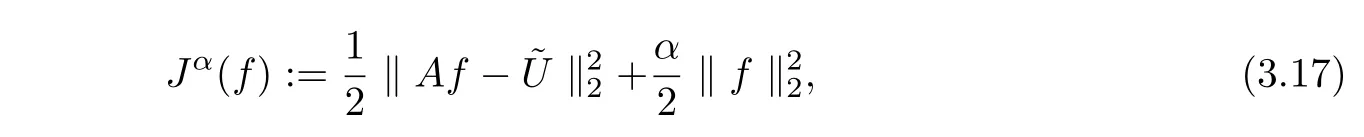
where 0＜α＜1 is the so-called regularization parameter,‖·‖2denotes the EuclideanL2-norm.

Equation(3.17)can be realized in discrete form using finite difference method,and then the gradient descent algorithm can be applied to solve the minimization problem[14].Details about computational issues are given in the next section.

§4.Numerical Experiments

In this section,we give several numerical experiments for recovery of the implied volatility.In our tests,we assumeT=1,R=0.05,K=100,a=0.892,σ0=0.02,θ(t)=(0.001+0.1t)e−0.9t+0.009,λ(t)=1−t,Λ =[0.01,0.04]and the noisy data takes the form

wherezstands for uniformly distributed random numbers and we chooseδ=0.01,0.05.

Firstly a mesh is generated withN=101 grid points on the interval[0,T]andM=51 grid points on the interval[0,R],then we use the finite differences method to solve the direct problem(1.5)～(1.6)with artificial boundary conditions that is∂V/∂r=0 atr=0 andR.

The equation(3.16)can be discretized as following

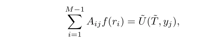
whereAij=P(ri,yj)∆r(ri∈[0,R],∆r=R/M),yj=rje−aT+c(T)withrj∈Λ.Here we generate 61 grid points on the interval Λ.

In order to solve the problem(3.17),we take a fixed valueα=0.001 and use the gradient descent method.We consider the perturbation function obeys the linear distribution,the sine distribution and the piecewise function respectively.For the first one,we let the functionf(r)=εr,for the second one,we letf(r)=εsin(40πr),and for the last,we letf(r)=εforr∈[0,0.02]∪(0.04,0.05],andf(r)=0 forr∈(0.02,0.04].According to different perturbation functions,we choose different values ofεto make the perturbations can reach 0-0.5 of the magnitude of constant volatilityσ0.

Example 1f(r)=εr.With differentε=0.001,0.0025,0.005,0.01,we can obtain the reconstructed perturbation functions.Figures 1,2 show the reconstructed results and relative errors respectively.From Figure 2,we obtain that smallerεyields smaller relative errors and gives better reconstruction.It can be seen from the equation(2.2)that the linearization procedure(3.4)gives more accurate approximation to the original nonlinear inverse problem if the parameterεis smaller.

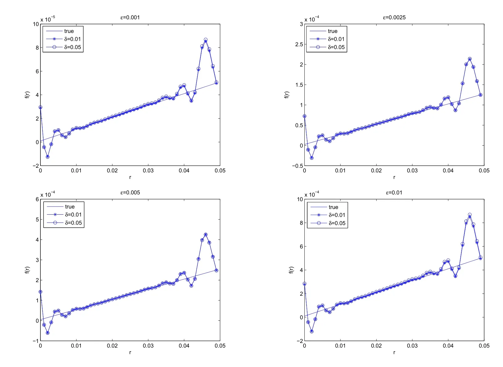
Figure 1 Reconstructed Perturbation with Different Parameters of ε

Example 2f(r)=εsin(40πr).For this example,we consider different parameters ofε=0.001,0.0025,0.005,0.01.Figures 3,4 show the reconstructions and relative errors respectively.Clearly,we can see that whenε=0.001,the reconstruction result is the most close to the true value.

Example 3In this example,the functionf(r)is discontinuous and we let the parameters ofε=0.001,0.0025,0.005,0.01.Figures 5,6 show the reconstructions and relative errors respectively.From the figures,we can get the same result as the above two examples.In this case,the errors between the estimated results and the true value are relatively large.Also we can see that at the discontinuous pointsr=0.02 and 0.04,the errors reach maximum.For this situation that the perturbation is non-smooth,our future work is to apply the total variation regularization method to reconstruct the volatility more accurately.

Furthermore,in this paper,we consider volatility depend on interest rate only.In the next step,we will consider the case that volatility doesnot depend on interest rate,but also relates to the time and text our algorithm to the real market data.

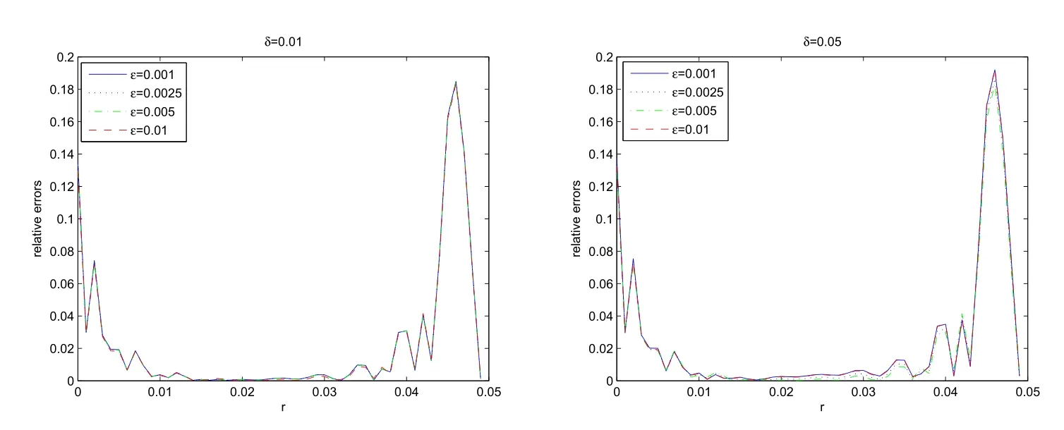
Figure 2 Relative Errors with Different Parameters of ε

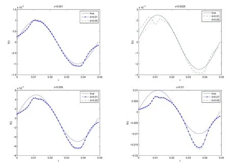
Figure 3 Reconstructed Perturbations with Different Parameters of ε

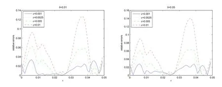
Figure 4 Relative Errors with Different Parameters of ε

Figure 5 Reconstructed Perturbations with Different Parameters of ε

Figure 6 Relative Errors with Different Parameters of ε

§5.Conclusion

In this paper,we study a numerical method for the reconstruction of the implied volatility in short-term interest rate model from the market prices of zero-coupon bonds.Assuming the volatility function to be combination of a given constant and a small perturbation,we simplify the partial differential equation.Introducing the power series,we derive recursive formulas of the price of zero-coupon bond.Then we consider the inverse problem by neglecting the high order terms in the power series,and obtain an integral equation of the perturbation function.In order to solve the inverse problem,we address the Tikhonov regularization method.Using the gradient decent method,three examples are considered and the numerical results show that the method is effective.In the test,by considering different values of the parameter in perturbation function,we get the result that smaller perturbation yields better reconstruction.

[1]HULL J.Options,Futures and Other Derivatives[M].New Jersey:Prentice Hall,2006.

[2]COX J C,INGERSOLL J E,ROSS S A.A theory of the term structure of interest rates[J].Econometrica,1985,53(2):385-408.

[3]HULL J,WHITE A.The general Hull-White model and super calibration[J].Finance Analysis Journal,2001,57(6):34-43.

[4]BOUCHOUEV I,ISAKOV V.The inverse problem of option pricing[J].Inverse Problems,1997,13(5):11-17.

[5]BOUCHOUEV I,ISAKOV V.Uniqueness,stability and numerical methods for the inverse problem that arises in financial markets[J].Inverse Problems,1999,15(3):95-116.

[6]ZHANG Guan-quan,LI Pei-jun.An Inverse Problem of Derivative Security Pricing[C].New Jersey:The International Conf on Inverse Problems,World Sci,2003:411-419.

[7]EGGER H,HEIN T,HOFMANN B.On decoupling of volatility smile and term structure in inverse option pricing[J].Inverse Problem,2006,22(4):1247-1259.

[8]EGGER H,ENGL H W.Tikhonov regularization applied to the inverse problem of option pricing:convergence analysis and rates[J].Inverse Problems,2005,21(3):1027-1045.

[9]RAINER M.Calibration of stochastic models for interest rate derivatives[J].2009,58(3):373-388.

[10]BOUCHOUEV I,ISAKOV V,VALDIVIA V.Recovery of volatility coefficient by linearization[J].Quantitative Finance,2002,2(4):257-263.

[11]LU Lu,YI Lei.Recover implied volatility of underlying asset from European option price[J].Journal of Inverse and Ill-posed Problems,2009,17(5):499-509.

[12]HULL J,WHITE A.Pricing interest-rate-derivative securities[J].The Review of Financial Studies,1990,3(4):573-592.

[13]BAO Gang,LI Pei-jun.Near- field imaging of in finite rough surfaces in dielectric media[J].SIAM J.Imaging Sciences.2014,7(2):867-899.

[14]WANG Yan-fei.Computational Methods for Inverse Problems and Their Applications[M].Beijing:Higher Education Press,2007.