
Compressible effect on the cavitating flow: A numeric study *
2017-03-14 07:06WeiZhang张伟XiaodongBai柏晓东ZhengMa马峥GangChen陈刚YongWang
水动力学研究与进展 B辑 2017年6期
Wei Zhang (张伟), Xiao-dong Bai (柏晓东), Zheng Ma (马峥), Gang Chen (陈刚), Yong Wang
1. Science and Technology on Water Jet Propulsion Laboratory, Marine Design and Research Institute of China,Shanghai 200011, China, E-mail: waynezw0618@163.com
2. Ministry of Education Key Laboratory of Structural Dynamic Behavior and Control, School of Civil Engineering, Harbin Institute of Technology, Harbin 150090, China
3. China Ship Scientific Research Center, Wuxi 214082, China
4. Max Planck Institute for Dynamics and Self-Organization, Am Faßberg 17, Göttingen 37077, Germany
Phase change from liquid to vapor in the lowpressure region is the main feature of the cavitation. If the low-pressure region is located at downstream of a bluff body, the cavitation produced by separation could be unstable. Such phenomenon is believed to be characterized by the re-entrant jets[2,3], as shown in Fig.1(a). Many experimental measurements have been carried out to study the re-entrant jets and the cavitation[4-6]. Most recently, Ganesh et al.[7]found experimentally bubbly shock propagation, as shown in Fig.1(b), indicating that compressibility of the bubbly mixture could be another key factor of unstable cavitation.
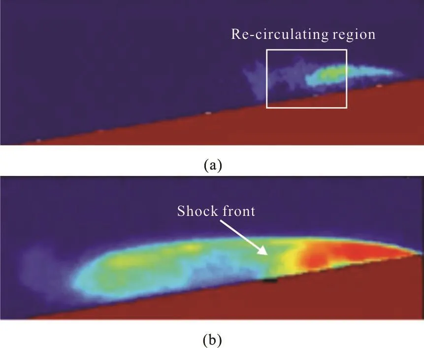
Fig.1 (Color online) Two different types of unstable cavitation on the wedge, from the supplemental material of Ref.[5]
Although there are many numerical simulations carried out to study the cavitation, only a few considered the compressibility. Goncalvès developed a onefluid compressible Reynolds averaged Navier-Stokes(RANS) solver with a simple equation of state (EOS)based on a sinusoidal barotropic law for the mixture[8].He used the solver to compute a periodic unsteady cavitation on a wedge[9], and only re-entrant jet flow was captured. To the best of our knowledge, there is no published numerical work concerning the com-pressibility of the mixture in the cavitating flow so far.
To understand the compressible effect on the cavitating flow, the compressible, multiphase, single component RANS solver, cavitatingFoam, developed by Karrholm et al.[10]within the open source CFD package, OpenFOAM, is used in the present work. To close the mathematic model, a barotropic EOS is chosen to link the pressure with the density. The barotropic EOSs for pure liquid and pure vapor are given below:

where the subscripts v and l refer to vapor and liquid respectively. ψ refers to the compressibility,and is the inverse square of the speed of sound C.The mixture of bubbly flow is assumed to be in homogenous equilibrium. The local fraction of the vapor, γ, is computed as below
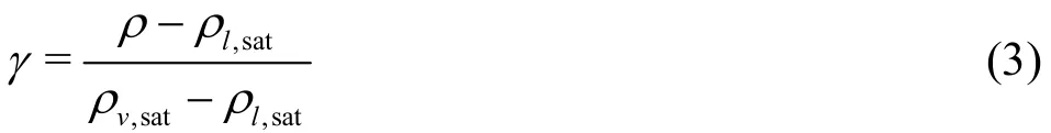
Karrholm et al.[10]used a linear interpolation function to calculate ψ for mixture based on the fraction of the vapor, γ. However, because of the complex nonlinear effect of the compressibility in the mixture, such linear interpolation may not be good enough. For instance, the speed of sound for water and water vapor are 1 480 m/s and 348 m/s respectively at 20oC, while that of the mixture can be as slow as 20 m/s. In other words, linear interpolation function does not represent the underlying physics and cannot be used to simulate the compressible effects of the bubbly mixture especially for cavitating flow under the influence of the compressibility. Brennen introduced a model by assuming the new equilibrium could be rapidly established when a small pressure change occurred in the mixture[11]. And according to his work,the compressibility ψ can be calculated based on the local volume fraction of vapor γ as below
Based on this equation, ψ can be plotted as a function of γ for diesel fuel. As shown in Fig.2, the local speed of sound could be slower than 20 m/s in the mixture. As a result, high local Mach number could be expected in the cavitating flow of diesel fuel even when the character speed is not too large. In fact,Ganesh et al.[7]used a modified version of this formula to estimate the local speed of sound in their measurement, and then got shock propagation as the conclusion.

Fig.2 Speed of sound as a function of vapor fraction
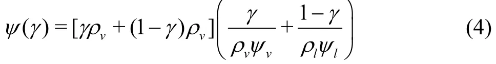
Fig.3 The schematic view of the domain
The Brennen’s model for speed of sound in the mixture is adopted here to simulate the cavitating flow on a wedge. Ganesh et al. performed experimental measurements for this case. The schematic view of the domain for the present simulation is given in Fig.3. A quasi-2D domain is considered in the present work.The length and the height of the wedge,WL andwh,are 180 mm and 25.4 mm respectively. The domain size Lx×Lyis 60LW×28LW. Ltand Lcare the Reynolds number, Re= UrefLW/ν, is set to be 1.44×10⁶, where ν is the kinematic viscosity of fuel.The cavitation number, σ = (Pref- Psat)/(0.5ρ U2), is maximum cavity thickness and the maximum cavity length, respectively. A mesh with 151 657 hexahedra cells is used here. The mesh is refined around the wedge region with refineMesh in OpenFOAM. Just one layer is considered in the 3rddirection, and the front and back directions are set to be empty boundary condition. A fixed valuerefU is given for velocity at the inlet of the domain. The pressure at the outlet boundary is set to be the reference pressurerefP .Diesel fuel is considered in our simulation. The set to be 1.95, wheresatP is the vapor pressure of diesel fuel. These two parameters are the same as those used in Ganesh et al.’s experiment. The speed of sound for the liquid and the vapor are set to be 1 414 m/s and 632 m/s respectively. The SST -kω model is used to model the turbulence.
Firstly, the maximum cavity lengthcL and thicknesstL from the present work and literatures are compared in Fig.4 for validation. It is shown that the numerically obtained maximum thickness agrees with the experimental result and analytical solution based on free-streamline theory in Ref.[7]. The maximum cavity length from present simulation is smaller than the measured result. By considering the measurement uncertainties in the reference, the current numerical results are acceptable. Moreover,we only focus on qualitative analysis rather than quantitative analysis in the present letter.
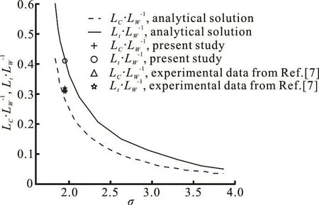
Fig.4 The simulated maximum cavity length as well as thickness, Compared with the measured ones and the analytical solutions with the free-streamline theory from Ref.[7]
The time series of the vapor fraction is shown in Fig.5. An unsteady cavitating flow can be observed in the numerical results. This flow pattern is similar to Ganesh et al.’s observation by referring to Fig.17 in Ref.[7]. A cavity is generated and grows from the apex of the wedge. During growing, the cavity is affected by the shear between the liquid and the vapor.So that a small amount of vapor at tip of the cavity starts to shed, as shown in Fig.5(b) for t=0.00097s .A cloud cavitation is formed there. Such shear flow is also given in Fig.6. No re-entrant jet is found during the shedding. The cavity keeps growing till it reaches the complete growth. In the meantime, the mount of shed cavitation cloud keeps increasing as well. That could be because of the vortex generated at the tip, as in the Kelvin-Helmholtz instability. As a result, the local pressure drops and the liquid vaporizes locally.After the complete growth, the cavity starts to shrink,and its left boundary moves from downstream to upstream as shown in Figs.5(d) and 5(e). Similar flow pattern has also been observed in the experiment(Fig.1(b)). It could also be seen from those figures that a bubbly mixture is formed between the shed cloud cavitation and the cavity. Finally the cavity is pinched off from the wedge apex.
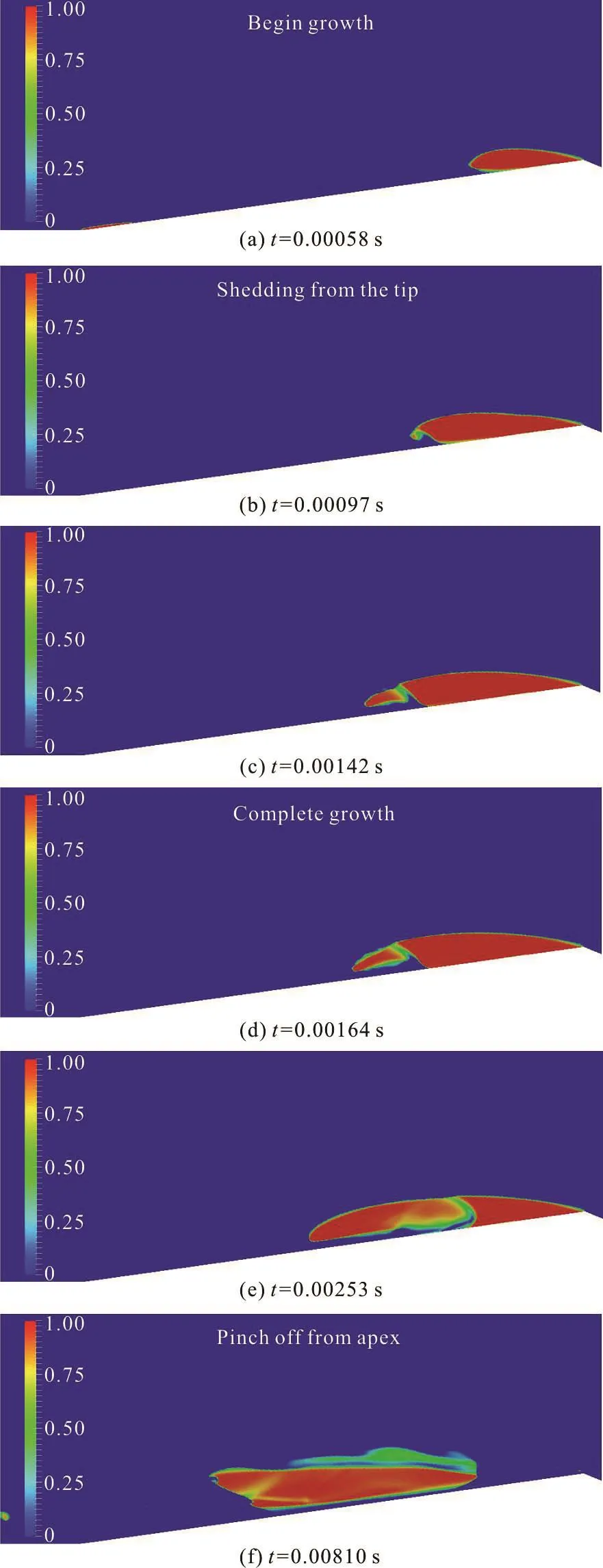
Fig.5 (Color online) Time series of the vapor fraction parameter γ within one cycle
To further understand the underlying physics, the compressibility parameter ψ and the local Mach number, which is defined as Ma = u/ C, are shown in Fig.7 for t =0.00253s.u is the magnitude of local velocity and C is local speed of sound. By referring to γ at the corresponding time point in Fig.6, a highly compressible region can be found in Fig.7(a) between the cavity and shed cavitation cloud.A green block on the left side of the cavity in Fig.7(b)represents the highly compressible cloud cavitation,due to small value of the local speed of sound (see Fig.7(a) for reference). The Ma within this region is greater than 1, similar as reported by Ganesh et al.[7].Two narrow red taps, which almost cover the boundary of the cavity and the shed cavitation cloud, can also be found in Fig.7(b). It should be noted that such taps are numerically introduced by interpolation between the regions of liquid and vapor. The pressure jump of the shock in the mixture, as reported in Ref.[7], is not found in our simulation. But considering the local Ma within the bubble mixture between the cavity and shed cloud cavitation, a shock could be expected here.
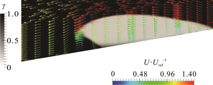
Fig.6 (Color online) Velocity field around the cavity at =t 0.00097s
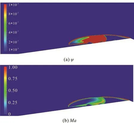
Fig.7 (Color online) The ψ and Ma at t=0.00253s
To explain such flow phenomenon, we propose that a Kelvin-Helmholtz instability, which induced by the shear between the liquid and vapor, results in a local pressure variation at the tip of the cavity. In the region where the pressure drops, the liquid is vaporized. It leads to further generation of the cloud cavitation in the downstream. Simultaneously the pressure increases on the boundary of the cavity. As a result,the cavity gets liquefied locally. A bubbly mixture keeps growing and the cavity shrinks within such region. As the bubbly mixture is highly compressible,shock could be happened in this region.
In summary, a compressible, multiphase, single component RANS solver is used to simulate the cavitating flow on a wedge in the present work. The barotropic equation of state is chosen for modeling the compressible effect. A non-linear model is used to predict the local speed of sound within the bubbly mixture. We observed in the numerical simulation an unsteady cloud cavitation phenomenon, which generates a highly compressible bubbly mixture. We propose that the unsteady cavitation phenomenon observed here is because of the instability of the cavity closure.The re-entrant jet could also induce the unsteady sheet-to-cloud cavitation. Both can be found under certain condition. But to the best of our knowledge, no criterion has been proposed so far to distinguish them.Further theoretical, numerical and experimental studies will be carried out to check the mechanism of both flow patterns.
[1] Luo X. W., Ji B., Tsujimoto Y. A review of cavitation in hydraulic machinery [J]. Journal of Hydrodynamics, 2016,28(3): 335-358.
[2] Zhang L. X., Zhang N., Peng X. X. et al. A review of studies of mechanism and prediction of tip vortex cavitation inception [J]. Journal of Hydrodynamics, 2015, 27(4): 488-495.
[3] Lush P. A., Skipp S. R. High speed cine observations of cavitating flow in a duct [J]. International Journal of Heat Fluid Flow, 1986, 7(4): 283-290.
[4] Bark G. Developments of distortions in sheet cavitation on hydrofoils [C]. ASME International Symposium on Jets and Cavities. Miami, Florida, USA, 1985, 470-493
[5] Le Q., Franc J. P., Michel J. M. Partial cavities: Global behavior and mean pressure distribution [J]. Journal of Fluids Engineering, 1993, 115(2): 243-248.
[6] Kawanami Y., Kato H., Yamaguchi H. et al. Mechanism and control of cloud cavitation [J]. Journal of Fluids Engineering, 1993, 119(4): 788-794.
[7] Ganesh H., Makiharju S. A., Ceccio S. L. Bubbly shock propagation as a mechanism for sheet-to-cloud transition of partial cavities [J]. Journal of Fluid Mechanics, 2016,802: 37-78.
[8] Goncalves E. Numerical study of unsteady turbulent cavitating flows [J]. European Jounral of Mechanics B/ Fluids, 2011, 30(1): 26-40.
[9] Decaix J., Goncalves E. Compressible effects modeling in turbulent cavitating flows [J]. European Jounral of Mechanics B/ Fluids, 2013, 39: 11-31.
[10] Karrholm F. P., Weller H., Nordin N. Modelling injector flow including cavitation effects for diesel applications[C]. Proceedings 5th Joint ASME/JSME Fluids Engineering Conference. San Diego, California USA, 2007.
[11] Brennen C. E. Cavitation and bubble dynamics [M].Oxford, UK: Oxford University Press, 1995.
猜你喜欢
Chinese Physics B(2022年8期)2022-08-31
Chinese Physics B(2022年8期)2022-08-31
Chinese Physics B(2022年4期)2022-04-12
Chinese Physics B(2022年1期)2022-01-23
金秋(2020年14期)2020-10-28
应用数学(2020年1期)2020-01-10
电影文学(2018年10期)2018-12-10
中华家教(2018年9期)2018-10-19
初中生世界·九年级(2017年10期)2017-11-08
中学生数理化·八年级数学人教版(2017年1期)2017-03-25
- 水动力学研究与进展 B辑的其它文章
- Bubbly shock propagation as a mechanism of shedding in separated cavitating flows *
- A sharp interface approach for cavitation modeling using volume-of-fluid and ghost-fluid methods *
- On the numerical simulations of vortical cavitating flows around various hydrofoils *
- Experimental measurement of tip vortex flow field with/without cavitation in an elliptic hydrofoil *
- The effect of water quality on tip vortex cavitation inception *
- Novel scaling law for estimating propeller tip vortex cavitation noise from model experiment *